Hopping conductivity of a suspension of flexible wires in an insulator

Abstract

We study the hopping conductivity in a composite made of Gaussian coils of flexible metallic wires randomly and isotropically suspended in an insulator at such concentrations that the spheres containing each wire overlap. Uncontrolled donors and acceptors in the insulator lead to random charging of wires and, hence, to a finite density of states (DOS) at the Fermi level. Then the Coulomb interactions between electrons of distant wires result in the soft Coulomb gap. At low temperatures the conductivity is due to variable range hopping of electrons between wires and obeys the Efros-Shklovskii (ES) law $\ln\sigma\propto-(T_{ES}/T)^{1/2}$ with $T_{ES}$ decreasing with concentration and length of the wires. Due to enhanced screening of Coulomb potentials, at large enough wire concentrations and sufficiently high temperatures, the ES law is replaced by the Mott law $\ln\sigma\propto-(T_{M}/T)^{1/4}$.

I Introduction

The electronic transport properties of composites made of metallic granules surrounded by some kind of insulator is widely studied. Spheroidal metallic particles or quantum dots Vinokur ; Gerber ; Jusz , relatively short carbon nanotubes Benoit ; Gaal ; Fuhrer ; Yosida , and long flexible nanowires such as bundles of carbon nanotubes or conducting polymers Heeger1 ; Kaiser ; Wessling are examples of the dispersed granules. If the concentration $n$ of the metallic granules is large, they touch each other and the conductivity is metallic. When $n$ is smaller than the percolation threshold $n_{c}$, the composites are in the insulating side of the metal-insulator transition and hopping is the only mechanism of conduction.

If each granule is neutral, adding or removing one electron from it costs a considerable electrostatic energy. The charge transport is blocked by this Coulomb charging energy and has activation dependence of the conductivity resembling the Arrhenius law. However it is generally observed that at low temperatures, the conductivity $\sigma$ exhibits a temperature dependent characteristic of variable range hopping (VRH) transport,

$$\sigma=\sigma_{0}\exp[-(T_{0}/T)^{\alpha}],$$ (1)

where $T_{0}$ is a characteristic temperature. For spheroidal particles or quantum dots Vinokur ; Gerber ; Jusz , $\alpha$ is observed to be $1/2$. For bundles of single wall carbon nanotubes Benoit , both $\alpha=1/2$ (Ref.  Benoit ) and $\alpha=1/4$ (Ref.  Benoit ; Gaal ; Fuhrer ; Yosida ) are reported. In composites made of conducting polymers dissolved in some kind of insulating polymer matrix Heeger1 ; Kaiser ; Wessling , the index $\alpha$ was found to be $1/2$ below the percolation threshold and at larger concentrations, $\alpha$ evolves from $1/4$ to $1$ (Ref. Heeger1 ). The finite DOS at the Fermi level necessary for the VRH conductivity is attributed to the charged impurities in the insulator playing the role of randomly biased gates. Then the interaction of electrons residing on different wires creates the Coulomb gap, which leads to ES VRH between granules Zhang ; Vinokur . In our recent paper nanotube , we studied the puzzling crossover from ES law with $\alpha=1/2$ to Mott law with $\alpha=1/4$ for a suspension of straight metallic wires. We showed that the characteristic temperature $T_{ES}\propto 1/(nL^{3})^{2}$, where $L$ is the wire length.

In this paper we would like to calculate the hopping conductivity for the more complicated case of flexible nanowires suspended in the insulating medium. They can be just very thin metallic wires suspended in an insulating liquid which was abruptly frozen, or very long single wall nanotubes or their bundles, or heavily doped conducting polymers. Such objects can have one or many parallel metallic channels. In the latter case, particularly for doped conducting polymers, disorder should be important and leads to localization of states at some distance along the nanowire Heeger . Nevertheless in this paper we concentrate on a fundamental problem of clean or weakly disordered wires. Generalization of our theory to the case of strongly disordered wires, where electrons are localized within distances much smaller than the wire length, will be discussed in the conclusion.

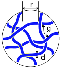
Figure 1: Local view of the semidilute solutions of flexible Gaussian wires. We show the case where the mesh size is not longer than persistence length, the wire within each mesh is essentially straight. At lesser density, the mesh size is longer than the persistence length, and then the wire in the mesh is wiggly (not shown).

We assume that each wire has the contour length $L$, relatively large persistence length $p$ and the diameter (thickness) $d$. We assume $L\gg p\gg d$. Throughout this work we require $L<p^{3}/d^{2}$ and this lets us disregard the effect of excluded volume, considering each wire as a Gaussian coil with the size $R=\sqrt{Lp}$. At small concentrations, where the inter-coil distance is much larger than the coil size, we can simply utilize the results for arrays of quantum dots Zhang . The overlap of the coils starts when the concentration of wires exceeds the concentration of the wire inside one coil: $n=1/(Lp)^{3/2}$ (see Fig. 1). Therefore our discussion is confined to the range of concentrations $1/(Lp)^{3/2}\ll n\ll n_{c}$, where $n_{c}=1/L^{2}d$ is the percolation threshold at which the hoppping conductivity is replaced by the metallic one (we derive the expression of $n_{c}$ below).

In this paper we restrict ourselves to the scaling approximation for the conductivity and to delineating the corresponding scaling regimes. In our scaling theory, we drop away both all numerical factors and, moreover, also all logarithmic factors, which do exist in the problem, because it deals with strongly elongated cylinders. In this context, we will use symbol “$=$” to mean “equal up to a numerical coefficient or a logarithmic factor”.

Our main results for the hopping conduction are presented by the phase diagrams in the plane of parameters $n(Lp)^{3/2}$ and $T$ shown in Figs. 2, 3 and 4. Fig. 2 represents the simplest case of narrow wires with only one conducting channel and relatively long length $p^{2}/d<L<p^{3}/d^{2}$. Remarkably the ES hopping regime which vanishes for single channel straight wires nanotube does exist for Gaussian coiled wires. The reason is that each straight wire is a one dimensional object where Coulomb interaction plays only marginal role. On the other hand, a coiled metallic wire from the point of view of the Coulomb interaction is a two-dimensional object, where charging energy $E_{c}$ can be substantially larger than the quantum level spacing $\delta$. At large enough $n(Lp)^{3/2}$ and sufficiently high temperature, ES hopping conductivity is replaced by the Mott law due to increasing screening of coulomb potentials (regime M). At even higher temperatures both VRH regimes crossover to the nearest neighbor hopping (NNH) regimes.

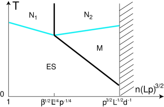
Figure 2: (Color online) Summary of scaling regimes for the case of flexible Gaussian coiled wires each with single conducting channel and length $p^{2}/d<L<p^{3}/d^{2}$. Dark line separates regimes where Coulomb interaction is important from regimes where it plays minor role. The grey (blue) line separates activated NNH regimes $\rm N_{1}$ and $\rm N_{2}$ from VRH regimes $\rm ES$ and $\rm M$.

The plan of this article is as follows. In Sec. II we first consider the macroscopic dielectric constant $\kappa_{\rm eff}$ of the suspension. We then calculate the finite DOS at the Fermi level in Sec. III. We continue in Sec. IV by calculating the effective localization length $\xi$ for hop over distances larger than the typical coil size. Using these results, we summarize all the scaling regimes for the hoping conductivities in Sec. V. Finally in Sec. VI, we conclude with the discussion of generalization of our theory to the case where wires are strongly disordered.

II Dielectric Constant

We start with determining the static macroscopic dielectric constant $\kappa_{\rm eff}$ of the suspension with wire concentration $1/L^{3}\ll n\ll n_{c}$. The percolation threshold $n_{c}$ can be estimated from the following argument. Percolation happens when each wire has roughly two direct contacts with other wires. Following Ref. Redbook , the number of contacts per wire is of the order of $nL^{2}d$ (each piece of the wire of the length $d$ has probability $nLd^{2}$ to be touched). Requiring that $nL^{2}d$ is of the order of 1, we obtain the percolation threshold $n_{c}=1/L^{2}d$. nematic

In Ref.conductivity , we have calculated the macroscopic conductivity $\sigma$ of a suspension of Gaussian coiled wires with conductivity $\sigma_{1}$ in a weakly conducting medium with conductivity $\sigma_{2}\ll\sigma_{1}$. When dealing with metal wires in an insulator, one can consider small final frequency response and use $-i\omega\kappa/4\pi$ for $\sigma_{2}$. This lets us find the macroscopic effective conductivity $\sigma(\omega)$ and $\kappa_{\rm eff}$ using $\kappa_{\rm eff}=4\pi i\sigma(\omega)/\omega$,

$$\kappa_{\rm eff}=\left\{\begin{array}[]{lcr}\kappa n^{2}L^{3}p^{3}&{\rm if}&1<n(Lp)^{3/2}<\frac{L^{1/2}}{p^{1/2}}\\ \\ \kappa nL^{2}p&{\rm if}&\frac{L^{1/2}}{p^{1/2}}<n(Lp)^{3/2}<\frac{p^{3/2}}{L^{1/2}d}\end{array}\right.\ ,$$ (2)

where $\kappa$ is the dielectric constant of the insulator. We notice that the polarization of these metallic wires leads to great enhancement of the macroscopic dielectric constant $\kappa_{\rm eff}$ much larger than $\kappa$ of the insulating host. The derivation of Eq. (2) is based upon the geometrical properties of the system, therefore let us dwell on them first.

In the parlance of polymer science, when wires strongly overlap at $n>1/(Lp)^{3/2}$, we deal with a semidilute solution - the system locally looks like a network with certain mesh size $r$ (see Fig. 1). In the scaling sense, $r$ is the same as the characteristic radius of density-density correlation function, and can be estimated following Ref. Redbook . Suppose that the wire within each mesh has a contour length $g$. It makes a density about $g/Lr^{3}$ which must be about the overall average density $n$. Thus, $g/Lr^{3}=n$. Second relation between $g$ and $r$ depends on whether mesh size is bigger or smaller than persistence length $p$:

$$r=\left\{\begin{array}[]{lcr}g&{\rm if}&g<p\\ \sqrt{gp}&{\rm if}&g>p\end{array}\right.\ .$$ (3)

Accordingly, one obtains

$$\begin{array}[]{lccr}g=\frac{1}{n^{2}L^{2}p^{3}}\ ,&r=\frac{1}{nLp}&{\rm if}&\frac{1}{(Lp)^{3/2}}<n<\frac{1}{Lp^{2}}\\ g=\sqrt{\frac{1}{nL}}\ ,&r=\sqrt{\frac{1}{nL}}&{\rm if}&\frac{1}{Lp^{2}}<n<\frac{1}{L^{2}d}\end{array}\ ,$$ (4)

The upper line corresponds to such a dense network that every mesh is shorter than persistence length and wire is essentially straight within each mesh (see Fig. 1). The lower line describes much less concentrated network, in which every mesh is represented by a little Gaussian coil.

Now we present a simple derivation of Eqs. (2) equivalent to what we have done for the macroscopic conductivity in Ref.conductivity . Consider a cube of the size about $(Lp)^{1/2}$ inside our macroscopic sample. On the one hand, the overall dielectric constant on the scale of this cube is already about the same as that of a macroscopic body, we denote it $\kappa_{\rm eff}$. Therefore the capacitance of such a cube is about $(Lp)^{1/2}\kappa_{\rm eff}$. On the other hand, we can estimate this capacitance considering wires inside the cube. Because the distance between wires is about $r$, each wire bridges another wire through a blob of insulator with size $r$ and capacitance $r\kappa$. Since the contour length of the wire inside each blob is about $g$, there are about $L/g$ such capacitors connected in parallel, yielding overall capacitance connecting the given wire as $(L/g)(r\kappa)$. Since all (or sizeable fraction of all) $n(Lp)^{3/2}$ wires in the cube are in parallel, we finally arrive at the cube capacitance as $n(Lp)^{3/2}(L/g)(r\kappa)$. Equating this to $(Lp)^{1/2}\kappa_{\rm eff}$ and accounting for the different geometrical properties represented by Eqs. (4), we arrive at Eq. (2).

Eqs. (2) can also be understood along the following way. If the wave vector $q$ is larger than $1/(Lp)^{1/2}$, the static dielectric function for the wire suspension has the metal-like form

$$\epsilon(q)=\kappa\left(1+\frac{1}{q^{2}r^{2}}\right),$$ (5)

where $r$ represents the typical separation of the wire from other wires and plays the role of screening radius for the wire charge. The function $\epsilon(q)$ grows with decreasing $q$ until $q=1/(Lp)^{1/2}$ where the composite loses its metallic response and $\epsilon(q)$ saturates. As a result, the macroscopic effective dielectric constant is given by $\kappa_{\rm eff}=\epsilon(q=1/(Lp)^{1/2})$. Plugging proper $r$ at different concentrations (Eq. (4)), we obtain $\kappa_{\rm eff}$ represented by Eqs. (2). They show how $\kappa_{\rm eff}$ grows with $L$ at $L\gg p$ for flexible nanowires. In the following sections, we will use Eqs. (2) for the calculation of the hopping conductivity. Note, however, that the dielectric constant of our system may be itself of interest in applications where very large dielectric constants are welcomed.

III Density of States

As we mentioned in the introduction, according to Ref. Zhang , the finite density of states (DOS) near the Fermi level originates from uncontrollable donors (or acceptors) in the insulating host. Donors have the electron energy above the Fermi energy of wires. Therefore, they donate electrons to wires. A positively charged ionized donor can attract and effectively bind fractional negative charges on all neighboring wires, leaving the rest of each wire fractionally charged. At a large enough average number ($\gg 1$) of donors per wire, effective fractional charges on different wires are uniformly distributed from $-e/2$ to $e/2$. In such a way the Coulomb blockade in a single wire is lifted and the discrete density of states get smeared. If the charging energy $E_{c}$ for a coil is larger than the mean quantum level spacing $\delta$ inside the wire, the DOS $g_{0}$ is given by $g_{0}=1/E_{c}(Lp)^{3/2}$. Substituting the effective dielectric constants given by Eqs. (2), we obtain the charging energy

$$E_{c}=\left\{\begin{array}[]{lcr}e^{2}/(\kappa n^{2}L^{7/2}p^{7/2})&{\rm if}&1<n(Lp)^{3/2}<\frac{L^{1/2}}{p^{1/2}}\\ \\ e^{2}/(\kappa nL^{5/2}p^{3/2})&{\rm if}&\frac{L^{1/2}}{p^{1/2}}<n(Lp)^{3/2}<\frac{p^{3/2}}{L^{1/2}d}\end{array}\right.\ .$$ (6)

In the very vicinity of the Fermi energy, the long range Coulomb interaction creates the parabolic Coulomb gap $\Delta$ which leads to the ES VRH.

If $E_{c}$ is smaller than the mean quantum level spacing $\delta$, the Coulomb interaction plays minor role. The density of states $g_{0}$ becomes $1/\delta(Lp)^{3/2}$. Level spacing $\delta$ strongly depends on the cross section of the wire. If the wire is so narrow that it has only one conducting channel, $\delta$ is the order of $\hbar^{2}/m\lambda_{F}L$, where $\lambda_{F}$ is the Fermi wavelength and $m$ is the effective electron mass. In order to compare with the charging energy $E_{c}$, we introduce constant $\beta=\lambda_{F}/a$ and rewrite $\delta$ as $e^{2}/\beta\kappa L$. Most likely, $\beta$ is the order of $1$. If the wire is thick enough, the electrons have three dimensional energy dispersion and $\delta$ is the order of $\lambda_{F}\hbar^{2}/mLd^{2}$ or $\beta e^{2}a^{2}/\kappa d^{2}L$. For both cases, the ratio $E_{c}/\delta$ decreases with growing $n$ or $L$ because of enhanced screening of Coulomb interaction in a denser system of longer wires. To calculate the VRH conductivity, we need now another key quantity–the localization length $\xi$.

IV Localization Length

It was suggested Boris that long range hopping process exceeding the size of a single wire can be realized by tunneling through a sequence of wires. The states of the intermediate wires participate in the tunneling process as virtual states. The virtual electron tunneling through a single granule is called co-tunneling Nazarov ; Ioselevich ; Beloborodov ; Vinokur ; Fogler1 and regarded as a key mechanism of low temperature charge transport via quantum dots. One should distinguish the two co-tunneling mechanisms, elastic and inelastic. During the process of elastic co-tunneling, the electron tunneling through an intermediate virtual state in the granule leaves the granule with the same energy as its initial state. On the contrary, the tunneling electron in the inelastic co-tunneling mechanism leaves the granule with an excited electron-hole pair behind it. Which mechanism dominates the transport depends on the temperature. Inelastic co-tunneling dominates at $T>\sqrt{E_{c}\delta}$, while below this temperature, elastic co-tunneling wins. In discussions below, we consider sufficiently low temperatures such that only elastic co-tunneling is involved.

Let us remind the idea of the calculation of the localization length $\xi$ used in Ref. Boris ; Zhang ; Fogler . When an electron tunnels through the insulator between wires at the nearest neighboring hopping (NNH) distance $r_{n}$, it accumulates dimensionless action $r_{n}/a$, where $a$ is the tunneling decay length in the insulator. We want to emphasize that the NNH distance $r_{n}$ is realized only in one point of the wire and, therefore, is much shorter than the typical separation along the wire from other wires $r$. NNH distance $r_{n}$ can be calculated using the percolation method ES . If one consider each wire with thickness $r_{n}$, using the same idea we showed above, percolation through these cylinders appears, when $nL^{2}r_{n}=1$. Thus $r_{n}=1/nL^{2}$. Since we assume the metallic wire is only weakly disordered, we neglect the decay of electron wave function in the wire. Over distance $x$, electron tunnels $x/(Lp)^{1/2}$ times accumulating a dimensionless action of the order of $r_{n}/a$ each time. Thus, its wave function decays as $\exp[-xr_{n}/(Lp)^{1/2}a]=\exp(-x/\xi)$, where the localization length

$$\xi=a(Lp)^{1/2}/r_{n}=a(nL^{5/2}p^{1/2}).$$ (7)

Now we have all the elements needed to construct our phase diagrams of the conductivity at various temperatures and concentrations.

V Summary of Phase Diagrams

We first consider narrow wires each with only one conducting channel. Depending on the relation between $L$ and $p$, percolation can start before or after $n(Lp)^{3/2}=(L/p)^{1/2}$, where the Gaussian coiled wire within each mesh becomes straight at higher concentrations. Our results for these two cases are summarized in Figs. 2 and 3 in the plane of parameters $n(Lp)^{3/2}$ and $T$. Each line represents a smooth crossover except the percolation threshold $n(Lp)^{3/2}=p^{3/2}/L^{1/2}d$, where the insulator-metal transition happens. In the vicinity of this transition, the conductivity has a critical behavior, which goes beyond the scope of our scaling approach.

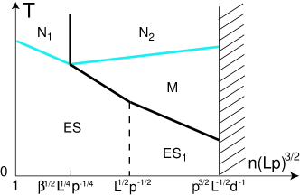
Figure 3: (Color online) Summary of scaling regimes for the case of flexible Gaussian coiled wires each with single conducting channel and length $p<L<p^{2}/d$. The dashed line marks the border where the wire within each mesh changes from Gaussian coiled to be straight. The effective dielectric constant $\kappa_{\rm eff}$ also changes at this line.

To be systematic, let us start the review of scaling regimes from Fig. 2, which is valid when $p^{2}/d<L<p^{3}/d^{2}$ and therefore percolation happens at relatively dilute solution with Gaussian coiled wire inside each mesh. We begin with activated NNH hopping regimes $\rm N_{1}$ and $\rm N_{2}$ at sufficiently high temperatures. The temperature dependence of the conductivity is given by

$$\sigma\propto\exp\left(-\frac{1}{nL^{2}a}\right)\exp\left(-\frac{E_{A}}{T}\right),$$ (8)

where the first term is due to electron wave function overlap and in the second term $E_{A}=max\{E_{c},\delta\}$ is the activation energy at very small tunneling conductances. Here the charging energy $E_{c}$ should be taken from the upper line of Eq. (6). Due to enhanced screening of Coulomb potentials with growing $n(Lp)^{3/2}$, $E_{c}$ decreases. As a result, the activation energy $E_{A}$ evolves from $E_{c}$ in regime $\rm N_{1}$ to the quantum level spacing $\delta$ in regime $\rm N_{2}$ at $n(Lp)^{3/2}=\beta^{1/2}L^{1/4}/p^{1/4}$. The Eq. (8) is valid as far as the contribution of the activation is smaller than that of the overlap. When they are comparable at sufficiently low temperatures, the NNH regimes smoothly crossover to VRH regimes at $T=e^{2}a/\kappa nL^{3/2}p^{7/2}$ and $T=e^{2}anL/\beta\kappa$ for the regimes $\rm N_{1}$ and $\rm N_{2}$ respectively.

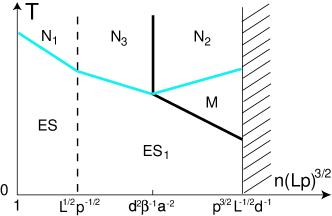
Figure 4: (Color online) Summary of scaling regimes for the case of thick wires with length $p<L<p^{2}/d$.

In the regime $\rm ES$, Coulomb interaction is important, which leads to the Efros-Shklovskii (ES) VRH conductivity

$$\sigma=\sigma_{0}\exp[-(T_{ES}/T)^{1/2}],$$ (9)

where $T_{ES}=e^{2}/\kappa_{\rm eff}\xi$. Applying the above line of Eqs. (2) and Eq. (7), we obtain

$$T_{ES}=\frac{e^{2}}{\kappa n^{3}L^{11/2}p^{7/2}a}.$$ (10)

At large $n(Lp)^{3/2}$ and relatively high temperatures, the ES law is replaced by the conventional Mott law,

$$\sigma=\sigma_{0}\exp[-(T_{M}/T)^{1/4}],$$ (11)

where $T_{M}=1/g_{0}\xi^{3}$. Plugging in $g_{0}$ for the narrow wires and Eq. (7), we arrive at

$$T_{M}=\frac{e^{2}}{\beta\kappa n^{3}L^{7}a^{3}}.$$ (12)

The regime $\rm ES$ borders the regime M along the line $T=\beta e^{2}a/\kappa n^{3}L^{4}p^{7}$, which can be obtained by equating the Coulomb gap width $\Delta=\sqrt{g_{0}e^{6}/\kappa_{\rm eff}^{3}}$ to the Mott’s optimal band width $T^{3/4}/(g_{0}\xi^{3})^{1/4}$.

When the wire is so short that $p<L<p^{2}/d$, percolation happens at relatively dense system where the wire within each mesh is straight. As a result, to the right of the transition from the coiled mesh to the straight mesh at $n(Lp)^{3/2}=(L/p)^{1/2}$, the effective dielectric constant should be taken from the bottom line of Eq. (2). Thus for the regime $\rm ES_{1}$, the characteristic temperature $T_{ES}$ in Eq. (9) should be replaced by

$$T_{ES_{1}}=\frac{e^{2}}{\kappa an^{2}L^{9/2}p^{3/2}}.$$ (13)

The crossover from this new regime $\rm ES_{1}$ to the regime M is along the line $T=\beta e^{2}a/\kappa nL^{2}p^{3}$. It is worthwhile to emphasize that Coulomb interaction loses its importance for the NNH regimes at $n(Lp)^{3/2}=\beta^{1/2}(L/p)^{1/4}$ which is smaller than $(L/p)^{1/2}$, where the geometry of the mesh changes and thus so does the effective dielectric constant $k_{\rm eff}$. As a result, compared to Fig. 2, the regime $\rm ES_{1}$ is the only new regime added in Fig. 3. At $p=L$, Fig. 3 resembles the case of straight wires, the ES regimes almost vanish. Until now, we complete the review of phase diagrams for the narrow wires each with single conducting channel.

For thick wires, simply using the corresponding density of states discussed in the Sec. III, we obtain phase diagrams similar to those for the case of narrow wires, but with new borders between scaling regimes. Unlike narrow wires, there is a possibility that the geometry of the mesh changes when the Coulomb interaction is still important. Scaling regimes of this case is shown in Fig. 4. There is a new NNH regime $\rm N_{3}$ where the the conductivity is represented by Eq. (8) with activation energy $E_{A}$ given by the bottom line of Eq. (6). Replacing $p$ by $L$ in Fig. 4, we again recover the result we got for straight wires in Fig. 2 of Ref. nanotube .

VI Conclusion

In this paper we calculated the macroscopic dielectric constant and the hopping conductivity of a suspension of Gaussian coiled metallic wires in an insulator. We obtained a plethora of different scaling regimes. Our results are applicable to wires made of well conducting metals with relatively small disorder. They can also be generalized to the case of strongly disordered wires where electrons are localized at a distance $\lambda$ much smaller than the length of the wire $L$. To this end, one should proceed similar to what we have done for straight wires in the Ref.nanotube . To calculate $\kappa_{\rm eff}$, one can imagine that the disorder effectively cuts the wire into shorter metallic pieces each with length $\lambda$. Therefore, we can calculate $\kappa_{\rm eff}$ thinking about a suspension of metal wires with shorter lengthes $\lambda$ but larger concentration $nL/\lambda$. Resulting $\kappa_{\rm eff}$ depends on $\lambda$ and is much smaller than that of clean wires. Calculating the effective localization length $\xi$ similarly to Sec. IV, we should add the decay of electron wave functions along the wire. Taking into account the fractal properties of the wire, we arrive at a much smaller localization length than that of clean metal. Reduction of $\kappa_{\rm eff}$ and $\xi$ leads to much larger $T_{ES}$, $T_{M}$ and much smaller hopping conductivity. We can construct phase diagrams which topologically look similar to diagrams of Figs. 2, 3 and 4, but they are more complicated and we are not showing them here.

- (1) I. S. Beloborodov, A. V. Loptain, V. M. Vinokur, and K. B. Efetov, cond-mat/0603522.
- (2) A. Gerber, A. Milner, G. Deutscher, M. Karpovsky, and A. Gladkikh, Phys. Rev. Lett. 78, 4277 (1997).
- (3) L. Murawski, B. Koscielska, R. J. Barczynski, M. Gazda, and B. Jusz, Philos. Mag. B 80, 1093 (2000).
- (4) J. M. Benoit, B. Corraze, and O. Chauvet, Phys. Rev. B 65, 241405(R) (2002).
- (5) R. Gaal, J. P. Salvetat, and L. Forro, Phys. Rev. B 61, 7320 (2000).
- (6) M. S. Fuhrer, W. Holmes, P. Delaney, P. L. Richards, S. G. Louie, and A. Zettl, Synth. Met. 103, 2529 (1999).
- (7) Y. Yosida, and I. Oguro, J. Appl. Phys. 86, 999 (1999).
- (8) J. Zhang, and B. I. Shklovskii, Phys. Rev. B 70, 115317 (2004).
- (9) M. Reghu, C. O. Yoon, D. Moses, Paul Smith, A. J. Heeger, and Y. Cao, Phys. Rev. B 50, 13931 (1994).
- (10) C. K. Subramaniam, A. B. Kaiser, P. W. Gillberd, C. -J. Liu, and B. Wessling, Solid Stat. Comm. 97, 235 (1996).
- (11) B. Wessling, D. Srinivasan, G. Rangarajan, T. Mietzner, and W. Lennartz, Eur. Phys. J. E 2, 207 (2000).
- (12) Tao Hu, and B.I. Shklovskii, cond-mat/0604644.
- (13) A. J. Heeger, Rev. Mod. Phys. 73, 681 (2001).
- (14) A. Yu. Grosberg, and A. Khoklov, Statistical Physics of Macromolecules (AIP Press, New York, NY, 1994).
- (15) The nematic ordering of wires starts at a larger concentration . Percolation starts earlier than the nematic ordering, because percolation requires a couple of contacts per wire, while nematic ordering requires a contact per a smaller persistance length .
- (16) Tao Hu, A. Yu. Grosberg, and B. I. Shklovskii, Phys. Rev. B 73, 155434 (2006).
- (17) B. I. Shklovskii, Sov. Phys. Solid State 26, 353 (1984).
- (18) D. V. Averin, and Yu. V. Nazarov, Phys. Rev. Lett. 65, 2446 (1990).
- (19) M. V. Feigel’man, and A. S. Ioselevich, JETP Lett. 81, 277 (2005).
- (20) M. M. Fogler, S. V. Malinin, and T. Nattermann, cond-mat/0602008.
- (21) I. S. Beloborodov, A. V. Lopatin, and V. M. Vinokur, Phys. Rev. B 72, 125121 (2005).
- (22) M. M. Fogler, S. Teber, and B. I. Shklovskii, Phys. Rev. B 69, 035413 (2004)
- (23) B. I. Shklovskii, and A. L. Efros, Electronic Properties of Doped Semiconductors (Springer-Verlag, Berlin, 1984).