Discrete breathers in BEC with two- and three-body interactions in optical lattice

Abstract

We investigate the properties of discrete breathers in a Bose-Einstein condensate with three-body interactions in optical lattice. In the tight-binding approximation the Gross-Pitaevskii equation with periodic potential for the condensate wavefunction is reduced to the cubic-quintic discrete nonlinear Schrödinger equation. We analyze the regions of modulational instabilities of nonlinear plane waves. This result is important to obtain the conditions for generation of discrete solitons(breathers) in optical lattice. Also using the Page approach, we derive the conditions for the existence and stability for bright discrete breather solutions. It is shown that the quintic nonlinearity brings qualitatively new conditions for stability of strongly localized modes. The numerical simulations conform with the analytical predictions.

I Introduction

Discrete breathers are important eigenmodes of the nonlinear discrete and periodic systems and their existence has been predicted for such systems as optical waveguide arrays, array of Josephson junctions, magnetic chains etc rev ; rev_f ; Leder01 . Recently discrete breathers in array of Bose-Einstein condensates has attracted a great deal of attention Tromb01 ; Abd01a ; Kon04 ; Alfimov ; Kevr04 ; AK ; Morsh . The localized atomic matter wave in BEC in the optical lattice(a gap soliton) has been observed recently in Ober04 . The theoretical approaches mainly based on the analysis of the Gross-Pitaevskii equation with periodic potential and cubic mean field nonlinearity. It corresponds to taking into account elastic two-body interactions and the potential of optical lattice. The progress with Bose-Einstein condensates on the surface of atomic chips and in atomic waveguides involves strong compression of BEC and so to essential increasing the density of BECs. Then it pose the problem of the taking into account three-body interactions effects. This interaction represent interest also for the understanding of the fundamental limits for the functioning of devices using BEC Pu . The existence of three-body interactions can play important role in the condensate stability Abd01b ; Akhmediev . Recently 3-body interaction arising due to the Efimov resonance has been observed in an ultra-cold gas of cesium atoms Kraemer .

Thus represent interest to investigate properties of discrete breathers in BEC in optical lattices when two- and three-body interactions are taken into account. One of the interesting properties of this system is the existence of the gap-Townes solitonAS05 . In the tight-binding approximation(see a section below) we show that the GP equation with periodic potential can be reduced to the cubic-quintic discrete nonlinear Schrödinger(CQDNLS) equation. This regime occurs for the deep optical lattice, which is realized in typical experiments in the BEC.

For the generation of discrete breathers the modulational instability of nonlinear plane wave represent the possible mechanism. Thus in this paper in the section 3 we discuss the modulational instability in the CQDNLS equation, the stability region of the wave in the lattice. In section 4 we discuss the localized modes of the different symmetries and the conditions of their stability.

II The model

Let consider BEC with two and three body interactions in optical lattice and in highly anisotropic trap corresponding to quasi 1D geometry. The Gross-Pitaevskii equation is

$$i\hbar\psi_{t}=-\frac{\hbar^{2}}{2m}\nabla^{2}\psi+\frac{m}{2}(\omega_{\perp}^{2}\rho^{2}+\omega_{x}^{2}x^{2})+V_{opt}(\rho,x)-g_{1}|\psi|^{2}\psi-g_{2}|\psi|^{4}\psi,$$ (1)

where $g_{1},\,g_{2}$ are coefficients proportional to two- and three-body elastic interactions. For rubidium atoms it is expected that the three-body interaction is attractive and $|g_{3}|\sim 10^{-26}-10^{-27}$cm⁶/s Pu . Here $\omega_{\perp}\gg\omega_{x}$, $V_{opt}=V_{0}\sin^{2}(kx)R(\rho).$ We look for the solution of the form

$$\psi(r,t)=\phi_{0}(\rho)\phi(x,t),$$ (2)

where $\phi_{0}$ is the solution of the radial linear equation

$$\frac{\hbar^{2}}{2m}\nabla_{\rho}^{2}\phi_{0}+\frac{m}{2}\omega_{\perp}^{2}\rho^{2}\phi_{0}=\frac{1}{2}\hbar\omega_{\perp}\phi_{0}.$$ (3)

The solution for the ground state is

$$\phi_{0}=\sqrt{\frac{1}{\pi a_{\perp}^{2}}}\exp(-\frac{\rho^{2}}{2a_{\perp}^{2}}).$$

Multiplying both sides of the GP equation by $\phi_{0}$ and integrating over transverse variable $\rho$ we obtain the quasi 1D GP equation

$$i\hbar\phi_{t}=-\frac{\hbar^{2}}{2m}\phi_{xx}+(\frac{m}{2}\omega_{x}^{2}x^{2}+V_{0}\sin^{2}(kx))\phi-\frac{g_{1}}{2\pi a_{\perp}^{2}}|\phi|^{2}\phi-\frac{g_{2}}{3\pi^{2}a_{\perp}^{4}}|\phi|^{4}\phi.$$ (4)

Introducing the dimensionless variables

$$t=t\nu,x=kx,\phi=u\sqrt{\frac{2a_{s}\omega_{\perp}}{\nu}},\nu=\frac{E_{R}}{\hbar},$$

where $E_{R}=\hbar^{2}k^{2}/2m$ is the recoil energy, we obtain the equation

$$iu_{t}+\frac{1}{2}u_{xx}+\lambda|u|^{2}u+\bar{\lambda}|u|^{4}u-V_{0}\cos(2x)u=0.$$ (5)

where $\lambda=\pm 1$ and

$$\bar{\lambda}=\frac{g_{2}}{3\pi^{2}\hbar\nu a_{\perp}^{4}}\left(\frac{\nu}{2a_{s}\omega_{\perp}}\right)^{5/2}.$$

In the case of deep optical lattice ($U\gg E_{R}$ i.e. $\nu\gg 1$) the tight-binding approximation can be used Tromb01 ; Abd01a ; Kon04 ; Alfimov . If the potential $U(x)$ periodic, i.e. $U(x+l)=U(x)$, the eigenvalue problem is:

$$\frac{d^{2}\phi_{\alpha,q}}{dx^{2}}+U(x)\phi_{\alpha,q}=E_{\alpha,q}\phi_{\alpha,q},$$ (6)

where for the optical lattice potential $U(x)=V_{0}\cos(2x)$. Here $\phi_{\alpha,q}$ is the Bloch function, $\alpha$ is the index labelling the energy bands $E_{\alpha}(q)$. Periodicity of the lattice admits the expansion of the energy

$$E_{\alpha,q+q_{0}}=E_{\alpha,q}=E_{\alpha,-q},\ q_{0}=\frac{2\pi}{l}.$$

Thus we can expand the energy in the Fourier series

$$E_{\alpha,q}=\sum_{n}\hat{\omega}_{n,\alpha}e^{iqnl},\ \hat{\omega}_{n,\alpha}=\frac{l}{2\pi}\int_{-q_{0}/2}^{q_{0}/2}E_{q,\alpha}e^{-iqnl}dq.$$ (7)

For deep lattice case it is convenient to use the Wannier functionsAlfimov :

$$w_{n,\alpha}=\sqrt{\frac{l}{2\pi}}\int_{-q_{0}/2}^{q_{0}/2}\phi_{\alpha,q}(x)e^{-iqnl}dq,$$ (8)

and

$$\phi_{\alpha,q}=\sqrt{\frac{l}{2\pi}}\sum_{n}w_{n,\alpha}(x)e^{iqnl}.$$ (9)

The main property of Wannier functions that they are strongly localized in the bottoms of the potential and so are suitable for the description of strongly localized modes in the periodic potential. They form an orthonormal and a complet set

$$\int_{-\infty}^{\infty}w_{n,\alpha}^{\ast}w_{n^{\prime},\alpha^{\prime}}(x)dx=\delta_{n,n^{\prime}}\delta_{\alpha,\alpha^{\prime}},$$

$$\sum_{n,\alpha}w_{n,\alpha}^{\ast}(x)w_{n,\alpha}(x^{\prime})=\delta(x-x^{\prime}).$$ (10)

Let look for the solution of CQ GP equation of the form of expansion in Wannier functions

$$u(x,t)=\sum_{n,\alpha}c_{n,\alpha}(t)w_{n,\alpha}(x).$$ (11)

Substituting this expansion into the GP equation (5) we obtain the system of equation for coefficients $c_{n,\alpha}$

$$ic_{n,\alpha;t} = \sum c_{n_{1},\alpha}\hat{\omega}_{n-n_{1},\alpha}+\lambda\sum_{\alpha_{1},\alpha_{2},\alpha_{3}}\sum_{n_{1},n_{2},n_{3}}c_{1}^{\ast}c_{2}c_{3}W^{nnnn}_{\alpha\alpha\alpha\alpha}+\bar{\lambda}\sum_{5\alpha}\sum_{5n}c^{\ast}_{1}c^{\ast}_{2}c_{3}c_{4}c_{5}W_{6\alpha}^{6n},$$ (12)

where

$$W_{nn_{1}n_{2}n_{3}}^{\alpha\alpha_{1}\alpha_{2}\alpha_{3}}=\int_{-\infty}^{\infty}w_{n,\alpha}w_{n_{1},\alpha_{1}}w_{n_{2},\alpha_{2}}w_{n_{3},\alpha_{3}}\ dx.$$

For deep optical lattice $V_{0}>5E_{R}$ are important terms with $n=n_{1}=n_{2}=n_{53}$ i.e. we are restricted by the band $\alpha$. Then the system is reduced for equation

$$iC_{n,\alpha;t}=\hat{\omega_{1,\alpha}}(C_{n-1,\alpha}+C_{n-1,\alpha})+\lambda W_{4\alpha}^{4n}|C_{n}|^{2}C_{n}+\bar{\lambda}W_{6\alpha}^{6n}|C_{n}|^{4}C_{n}.$$ (13)

By the transformation $v_{n}=C_{n,\alpha}\sqrt{W_{4\alpha}^{4n}}C_{n}$ this equation can be transformed into

$$iv_{n,t}+\kappa(v_{n+1}+v_{n-1})+\lambda|v_{n}|^{2}v_{n}+{\gamma}|v_{n}|^{4}v_{n}=0.$$ (14)

Here $\kappa=\hat{\omega_{1,\alpha}},\gamma=\bar{\lambda}W_{6\alpha}^{6n}/(2(W_{4\alpha}^{4n})^{2}).$ It is the cubic-quintic discrete nonlinear Schrödinger(CQDNLS) equation. As showed the analysis performed in Alfimov , the region of parameters exists, when the tight-binding approximation describes the GP equation with periodic potential with a high accuracy. It is achieved for the amplitudes of the periodic potential $|V_{0}|>5E_{R},\,$ and $E_{R}$ is the recoil energy. That corresponds to the experimentally realized values. When $\gamma=0$ the problem is reduced to considered previously by Tromb01 ; Abd01a ; Alfimov . In the recent work Malomed06 the case when $\lambda>0,\gamma<0$, motivated by the analysis of localized states in array of waveguides with saturable nonlinearity, has been considered. In the BEC case the parameter $\gamma$ can has any sign. The conserved quantities are: The norm(number of atoms) $N$ is:

$$N=\sum_{n}|v_{n}|^{2},$$ (15)

and the Hamiltonian $H$ is:

$$H=-\sum_{n=-\infty}^{\infty}\left[\kappa(v_{n}^{\ast}v_{n+1}+v_{n}v_{n+1}^{\ast})+\frac{\lambda}{2}|v_{n}|^{4}+\frac{\gamma}{3}|v_{n}|^{6}\right].$$ (16)

The equation of motion is:

$$iu_{n,t}=\frac{\delta H}{\delta u_{n}^{\ast}}.$$ (17)

The momentum is not conserved due to the discretness of the system. Due to the periodicity of the system the Hamiltonian is periodic with period $n=1$. The different excitations induces different effective periodic potential like the Peierls-Nabarro potential. The height of the barrier depends on the localization of the discrete soliton solution - grows with the decreasing of the soliton width. The analysis of the Hamiltonian can help for the calculation of the PN barrier between different discrete solitons and so help for the investigation of the stability of nonlinear modes Cai .

III Modulational instability of nonlinear plane waves

The nonlinear discrete equation has the plane wave solution

$$v_{n}(t)=\nu_{0}e^{i(qn+\omega t)},$$ (18)

with the dispersion relation

$$\omega=2k\cos q+\lambda{\nu_{0}}^{2}+\gamma{\nu_{0}}^{4}.$$ (19)

For special importance here are the staggered $q=\pi$ and unstaggered $q=0$ solutionsADG where the dispersion relation can be rewritten as

$$\omega=\pm 2k+\lambda{\nu_{0}}^{2}+\gamma{\nu_{0}}^{4}.$$ (20)

The linear stability of the solution (18) and (19) can be investigated by looking for a solution in the form

$$v_{n}(t)=(\nu_{0}+\delta v_{n}(t))e^{i(qn+\omega t)},$$ (21)

where $\delta v_{n}(t)$ is a small perturbation on the carrier wave, substituting (21) in (14) and keeping only the linear terms on $\delta v_{n}(t)$ and $\delta v^{\ast}_{n}(t)$ we obtain the following equation

$$i\delta v_{n,t}+k\cos q(\delta v_{n+1}+\delta v_{n-1}-2\delta v_{n})+(\lambda+2\gamma{\nu_{0}}^{2})(\delta v_{n}+\delta v^{\ast}_{n})=0.$$ (22)

Considering a modulation in the form

$$\delta v_{n}(t)=\left(\begin{array}[]{cc}\alpha\\ \bar{\beta}\end{array}\right)e^{i(Qn+\Omega t)},$$ (23)

where $Q$ and $\Omega$ are the wave number and the frequency of the linear modulation waves respectively then substituting it into (22) we obtain the following system of linear equations

$$i\Omega\alpha+4k\cos q\sin^{2}(Q/2)\bar{\beta}=0,$$

$$-(4k\cos q\sin^{2}(Q/2)+2(\lambda+2\gamma\nu_{0}^{2})\nu_{0}^{2})\alpha+i\Omega\bar{\beta}=0.$$ (24)

In order to have a nontrivial solution for the system the determinant of the coefficient matrix should be zero that leads to the following dispersion law

$$\Omega^{2}=8k\sin^{2}(Q/2)[2k\cos^{2}(q)\sin^{2}(Q/2)-\cos q(\lambda+2\gamma\nu_{0}^{2})\nu_{0}^{2}].$$ (25)

The plane wave solution (18) is modulationally unstable provided that $\Omega^{2}$ is negative and the gain is

$$G=2|\sin(Q/2)|\sqrt{2k\cos q(\lambda+2\gamma\nu_{0}^{2})\nu_{0}^{2}-2k\cos q\sin^{2}(Q/2))}.$$ (26)

From the gain equation we can see that the unstaggered solution $(q=0)$ are unstable whenever $\lambda\nu_{0}^{2}+2\gamma\nu_{0}^{4}>0$ and the staggered solutions $(q=\pi)$ are unstable whenever $\lambda\nu_{0}^{2}+2\gamma\nu_{0}^{4}<0$ which leads to the following cases:

i) $q=0$. If $\lambda>0$, $\gamma<0$ then we have MI of the unstaggered solution for $|\gamma|<\lambda/2\nu_{0}^{2}$ and if $\lambda<0$, $\gamma>0$ then we have MI when $|\gamma|>\lambda/2\nu_{0}^{2}$.

ii) $q=\pi$. If $\lambda>0$, $\gamma<0$ then we have MI of the staggered solution for $|\gamma|>\lambda/2\nu_{0}^{2}$ and if $\lambda<0$, $\gamma>0$ then we have MI when $|\gamma|<\lambda/2\nu_{0}^{2}$.

iii) In contradiction with the continuum case which is stable for the set of nonlinearities $\lambda<0$, $\gamma<0$ the staggered solution is modulationally instable regardless the value of any parameter. However the unstaggered solution should satisfy the inequality $\lambda\nu_{0}^{2}+2\gamma\nu_{0}^{4}>2k$, which is almost satisfied all the time for strongly localized modes, in order to have MI.

In the general case where $q$ can take any value we can distinguish two regions of MI as it is shown in Fig. 1 for positive $k\cos q$.

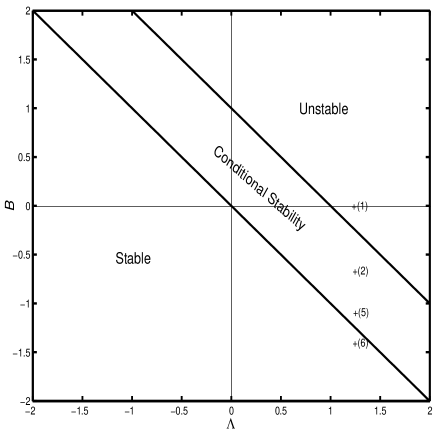
Figure 1: Modulational instability regions as function of the parameters $\Lambda=\gamma/2k{\nu_{0}}^{2}\cos q$ and $B=\beta/4{\nu_{0}}^{2}\cos q$. with $\cos q>0$, the labelled points are the points discussed in the text.

One is fully unstable and the other is conditional means it depends on the wave number $q$ of the carrier wave and the wave number $Q$ of modulation wave as it is shown in Fig. 2.

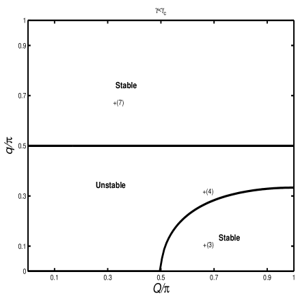
Figure 2: Regions of modulational instability in the plane $(q,Q)$ for the conditional stability region in Fig. 1, the labelled points are the points discussed in the text.

The conditional region represents the effect of the discreteness on the modulational instability. Clearly we can see that if we fix the cubic nonlinearity parameter and keep changing the quintic nonlinearity parameter then we will have instability, conditional instability and stability which shows that the quintic term can lead to collapse of MI. The role of quintic term also is very crucial on the wave numbers of the carrier and modulation waves leading to MI, where increasing $\gamma$ in the negative direction will shrink the MI region in $(q,Q)$ plane till a critical value $\gamma_{cr}$. This eliminates all possible chances to get MI then MI occurs again in the $(q,Q)$ plane in a mirror symmetry with the one occured for $\gamma<\gamma_{cr}$. In the continuum limit, when $Q<<1$ and $q<<1$ equation (25) reduced to

$$\Omega^{2}=2kQ^{2}[kQ^{2}/2-(\lambda+2\gamma\nu_{0}^{2})\nu_{0}^{2}]$$ (27)

and coincides with the one obtained in Darm98 . This MI gain does not depend on the wave number q of the carrier wave contrary to the discrete case.

Based on the analytical results, the modulational instabilities of carrier wave with wave number $q$ modulated by small oscillation with wave number $Q$ occurs when the right hand side of dispersion equation (25) is negative. In order to check our analytical results we have performed numerical simulations of equation (14) using fourth order Runge-Kutta scheme with a time step chosen to preserve our conserved quantities which are the total energy of the system and the number of atoms to accuracy more than 10^-4. The numerical simulations have been performed for a chain of $N=180$ units, with periodical boundary conditions so that the wave numbers $q$ and $Q$ satisfy the relations $q=2\pi m/N$ and $Q=2\pi M/N$, where $m$ and $M$ are integers. The other parameters have been chosen to be $k=0.1$, $\lambda=1$ with $\gamma$ varying, the amplitude of the modulation wave has been chosen small compared to the amplitude of the carrier wave as $\nu_{0}=0.5$, $\delta\nu_{0}=0.005$. The stability and instability regions as it was predicted by the analytical results has been checked for different points , starting with point labelled (1) in Fig.1 that correspond to zero quintic term with $q=Q=\pi/3$ and $q=\pi/3$, $Q=2\pi/3$. Our expectation of modulational instability has been confirmed as it is shown in Fig. 3 and independently from $q$ and $Q$.

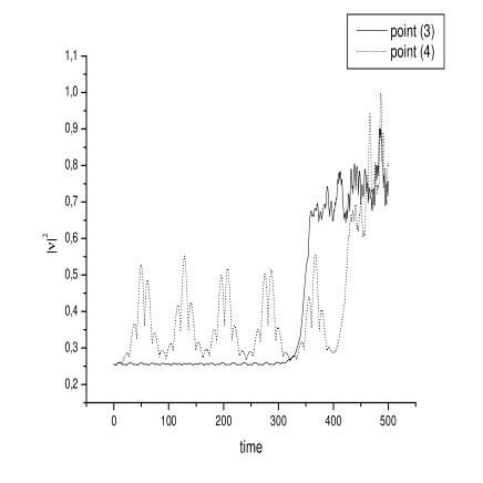
Figure 3: Modulational instability arises at different times at point labelled (3) started immediately and at the point labelled (4) the solution is stable for a long time before the occurrence of MI.

The role of discreteness investigated within the conditional instability region of Fig. 1 with quintic parameter $\gamma=-1.2$, where we choose two points: the point labelled (3) with $q=\pi/9$, $Q=2\pi/3$ and the point labelled (4) with $q=\pi/3$, $Q=2\pi/3$ from Fig.2 that correspond the same point labelled (2) in Fig. 1. The numerical results demonstrate the dependence of stability on $q$ and $Q$ as it is shown in Fig. 4.

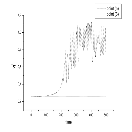
Figure 4: Modulational instability of the plane wave solution occurs and do not occurs at the same point in plane $(q,Q)$ with different $\gamma>\gamma_{c}$ $\gamma<\gamma_{c}$

IV Intrinsic localized modes(discrete breathers)

In this section we study the strongly localized solutions, which are standing and occupying few sites. In the case when the coupling between sites are weak the analytical approach can be used to find the discrete soliton (breather) solutions.

We used Page approach Page in order to examine the existence of the most known localized modes: even, twisted and odd modes(see Fig. 5). Twisted and even modes has been combined to one mode where both can be described by one formula as far as the evolution of one can be other after varying the quintic nonlinearity term.

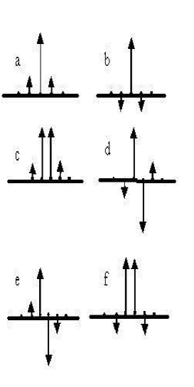
Figure 5: Schematic representation of different kind of odd modes (a unstaggered and b staggered), even modes (c unstaggered and d staggered)and twisted modes (e unstaggered and f staggered).

By considering solution for equation (14) as $v_{n}(t)=\nu_{n}{\rm e}^{(i\omega t)}$, where $\nu_{n}$ represents the respective amplitudes of a localized mode one can transform equation (14) to a system of algebraic equations depends on the topology of the localized mode, hence we derive the conditions of existence and then with linearization we derive the conditions of stability for each mode as follows.

Even mode

The even/twisted mode defined by its amplitudes as $v_{n}=\nu_{0}\left(\cdots,0,\alpha,1,s,s\alpha,0,\cdots\right)$ , where , $n=\pm 1,\pm 2,\cdots$, as we are concerned with the symmetric modes only $s=\pm 1$. Varying the signs of $s$ and $\alpha$ produces the different topologies of even/twisted modes showed in Fig. 5. Taking in consideration the requirements for strongly localized modes which are $|\alpha|\ll 1$ and $\alpha_{n}\approx 0$ for $n>2$ we derive the dispersion relation and the formula of the secondary amplitude respectively as

$$\omega \equiv \omega_{ET}=k(\alpha+s)+\nu_{0}^{2}(\lambda+\gamma\nu_{0}^{2}),$$ (28)

$$\alpha = \frac{k}{\nu_{0}^{2}(\lambda+\gamma\nu_{0}^{2})}.$$ (29)

Hence a set of conditions for existence of strongly localized modes can be derived as it is in table 1.

Mode	Existence conditions
Odd (a)	$\lambda>-\gamma\,\nu_{0}^{2}$
Odd (b)	$\lambda<-\gamma\,\nu_{0}^{2}$
Even (c) and Twisted (e)	$\lambda>-\gamma\,\nu_{0}^{2}$
Even (d) and Twisted (f)	$\lambda<-\gamma\,\nu_{0}^{2}$

Table 1: Conditions for existences of different kinds of modes shown in Fig. 5 and for positive coupling.

To study the stability of these modes we followed the approach developed in Darm98 by using a linear analysis, where we impose a perturbation $\delta_{n}(t)$ on each non zero excitation amplitude, hence the mode’s amplitude can be written now as

$$\nu_{n}=\nu_{0}(\cdots,0,r\alpha+\delta_{-2},1+\delta_{-1},s+\delta_{1},\alpha+\delta_{2},0,\cdots),$$

inserting it in (14) and with subsequent linearization we got eight-order system of equations. The change of variables as $\delta^{\pm}_{j}=\delta_{+j}\pm\delta_{-j}$ ($j$=1,2) reduces the system to two independent four-order equations systems. Separating the real and imaginary parts of the perturbation $\delta^{\pm}_{j}=\delta^{\pm}_{jr}+i\,\delta^{\pm}_{ji}$ and introducing the scaled time $\tau=\omega_{c}\,t$, we obtain

$$\frac{d\delta^{\pm}}{d\tau}=\left(\begin{array}[]{cccc}0&(s-p)\alpha&0&\alpha\\ 2-(3s-p)r\alpha+\displaystyle\frac{2\gamma\nu_{0}^{2}(1-r\alpha)}{(\lambda+\gamma\nu_{0}^{2})}&0&\alpha&0\\ 0&-\alpha&0&1\\ \alpha&0&-1&0\\ \end{array}\right)\delta^{\pm},$$ (34)

where $\delta^{\pm}=(\delta^{\pm}_{1r},\delta^{\pm}_{1i},\delta^{\pm}_{2r},\delta^{\pm}_{2i})$ and $p=\pm 1$ stands for the symmetric $\delta^{+}_{j}$ and antisymmetric $\delta^{-}_{j}$ perturbation respectively. If we introduce $\delta^{\mp}\propto{\rm exp}(g\tau)$ then the eigenvalues $g$ of (34) are given by the following equation

$$g^{4}+\left[1+\left(\frac{2\gamma\nu_{0}^{2}(p-s)}{(\lambda+\gamma\nu_{0}^{2})}+2(3-2ps)\right)\alpha^{2}+2(p-s)\left(1+\frac{\gamma\nu_{0}^{2}(p-s)}{\lambda+\gamma\nu_{0}^{2}})\right)\alpha\right]g^{2}$$

$$+2(p-s)\left(1+\frac{\gamma\nu_{0}^{2}}{\lambda+\gamma\nu_{0}^{2}}\right)\alpha+\left(2(3-2ps)+\frac{2\gamma\nu_{0}^{2}(1-p+s)}{\lambda+\gamma\nu_{0}^{2}}\right)\alpha^{2}$$

$$+\left(2(p-2s)-\frac{2\gamma\nu_{0}^{2}(1-p+s)}{\lambda+\gamma\nu_{0}^{2}}\right)\alpha^{3}+\alpha^{4}=0.$$ (35)

Hence similarly to the case without quintic nonlinearity Darm98 , when the symmetry of the mode coincides with the symmetry of perturbation that is $p=s$ the localized modes will be stable without any conditions on the nonlinearity parameters. In the case where the mode and the perturbation have different symmetries that $p=-s$ then there is a possibility for the mode to be unstable with the instability gain

$$g=-2\sqrt{1+\frac{\gamma\nu_{0}^{2}}{\gamma\nu_{0}^{2}+\lambda}}\sqrt{s\alpha}\left(1-\left(\frac{5s}{4}+\frac{\gamma\nu_{0}^{2}(1-2s)}{2(2\gamma\nu_{0}^{2}+\gamma)}\right)\alpha\right),$$ (36)

In contrast to the case of cubic nonlinearity only, where the mode is stable only when $\alpha s<0$, which means only twisted modes ( staggered and unstaggered ) are stable, it is clear in the cubic-quintic case that the first coefficient of (36) leads also to the possibility of stability of even modes (staggered and unstaggered) $\alpha s>0$. However taking the existence consideration only the unstaggered even mode is stable. The relationships between nonlinearities that control the stability is given in table 2.

Mode	Stability Conditions
Even (c & d)	$\lambda<-2\gamma\,\nu_{0}^{2}$
Twisted (e & f)	$\lambda>-2\gamma\,\nu_{0}^{2}$

Table 2: Conditions for stability of even/twisted modes showed in Fig. 1

In the numerical simulations, first we checked the stability of the even modes when the symmetry of the perturbation is the same as the symmetry of the mode. We found that the numerical results confirm the analytical predictions and the modes are stable always. For the case when the perturbation and the mode have opposite symmetry we checked the validity of analytically derived stability regions for the modes.

The most important result here is that the predicted stable even unstaggered mode, which is not possible in the case with cubic nonlinearity only, see Darm98 and references therein, has been demonstrated numerically see Fig. 6 for $\gamma=-0.6$ which is less than $\gamma=\lambda/2{v_{0}}^{2}=-0.5$. However when $\gamma=-0.4$ which is greater than $\gamma=\lambda/2{v_{0}}^{2}=-0.5$, the mode is unstable and it is transformed to the odd mode after some time as it is shown in Fig. 7. The even twisted modes are shown analytically to be stable within two different regions and this result has been checked numerically, which is in agreement with Darm98 for the case of cubic nonlinearity only.

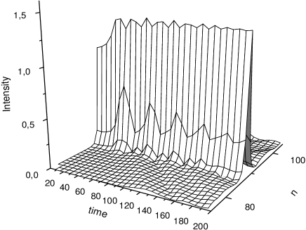
Figure 6: Evolution of perturbed unstaggered even mode (c) $\lambda=1,v_{0}=1,\gamma=-0.6$.

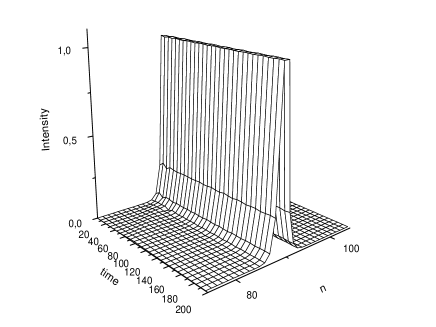
Figure 7: Evolution of perturbed unstaggered even mode (c) $\lambda=1,v_{0}=1,\gamma=-0.4$.

Odd mode

The odd mode is defined by its amplitude as $\nu_{n}=\nu_{0}(\cdots,0,\beta,1,s\beta,0,\cdots)$, where $n=0,\pm 1,\pm 2,\cdots$ and $s=\pm 1$ with the requirements for strong localized modes are $\beta\ll 1$ and $\beta_{n}\approx 0$ for $n>1$ and after performing similar algebraic operations to those done for even/twisted mode we obtain the dispersion relation and the formula of the secondary amplitude respectively as .

$$\omega \equiv \omega_{o}=k^{2}\frac{1+s}{\nu_{0}^{2}(\lambda+\gamma\nu_{0}^{2})}+\lambda\nu_{0}^{2}+\gamma\nu_{0}^{4},$$ (37)

$$\beta = \frac{k}{\nu_{0}^{2}(\lambda+\gamma\nu_{0}^{2})},$$ (38)

which leads to a set of conditions for the existence of this mode as it is shown previously in table 1. To study the stability of this mode we insert perturbation $\delta_{n}(t)$ on each non zero excitation amplitude as

$$\nu_{n}=\nu_{0}(\cdots,0,\beta+\delta_{-1},1+\delta_{0},s\beta+\delta_{1},0,\cdots),$$

then substitute it in equation (14) and perform linearization procedures, as we did for the even/twisted mode, we got a six-order system of equations, again a change of variables as $\delta_{1}^{+}=\delta_{+1}+\delta_{-1}$ reduces the system to four-order equations system. Separating the real and imaginary parts of the perturbation $\delta^{+}_{1}=\delta_{+1r}+i\,\delta_{1i}$ and $\delta_{0}=\delta_{0r}+i\,\delta_{0i}$, then introducing the scaled time $\tau=\omega_{c}t$ we obtain

$$\frac{d\delta^{\rm od}}{d\tau}=\left(\begin{array}[]{cccc}0&0&0&-\beta\\ 2+\displaystyle\frac{\gamma\nu_{0}^{2}}{\lambda+\gamma\nu_{0}^{2}}&0&\beta&0\\ 0&-2\beta&0&1\\ 2\beta&0&-1&0\end{array}\right)\delta^{\rm od},$$ (43)

where $\delta^{\rm od}=(\delta_{0r}^{\rm od},\delta_{0i}^{\rm od},\delta_{1r}^{\rm od},\delta_{1i}^{\rm od})$ . If we introduce $\delta^{\mp}\propto{\rm exp}(g\tau)$ then the eigenvalues $g$ of (43) are given by the following equation

$$g^{4}+\left[1+4s\beta\right]g^{2}+4\left[1+\frac{\gamma\nu_{0}^{2}}{\lambda+\gamma\nu_{0}^{2}}+\beta^{2}\right]\beta^{2}=0,$$ (44)

which have four roots and the one that control the stability is

$$g=\frac{1}{2}\sqrt{-2-8\beta^{2}+2\sqrt{1-24\beta^{2}+\frac{16\lambda\beta^{2}}{\lambda\nu_{0}^{2}+\lambda}}},$$ (45)

which shows that the instability gain Re($g$) will be a nonzero only if $|\beta|>\beta_{c}$ with $\beta_{c}=\displaystyle\pm\frac{1}{\sqrt{8}}\sqrt{\frac{\lambda+\gamma\nu_{0}^{2}}{\lambda+3\gamma\nu_{0}^{2}}}$. For $\gamma=\gamma_{c}=-\lambda/3\nu_{0}^{2}$, $\beta_{c}$ will be undefined, but we can conclude from equation (44) that the odd mode will be stable whatever the value of $\beta$. It is important to mention here that the value of $\beta_{c}$ is depend on the interplay between the cubic and quintic nonlinearities and satisfies the condition for strongly localized modes $\beta\ll 1$ for a range of values of these nonlinearities, in contrast to the case of the CDNLSE discussed in Darm98 where $\beta_{c}=1/\sqrt{8}$ which showed that the strongly localized mode is always stable because $\beta<\beta_{c}$ always. Furthermore for the stability of localized odd mode in CQDNLSE the condition $\gamma>\gamma_{c}=-\lambda/3\nu_{0}^{2}$ is necessary for focusing cubic nonlinearity and defocusing quintic nonlinearity. Finally we should mention here that for both even/twisted modes and odd modes cases, if we substitute $\gamma=0$ in our results, we get back to the cubic case and hence we reproduce the results of Darm98 . Numerical results for the case of odd modes presented in Figs. 8-9, confirmed the new predicted result that is the quintic nonlinearity term can lead to an unstable staggered odd mode when $-2<\gamma<-1.5$, this range is chosen to keep the mode strongly localized means the second amplitude $0.1\ \leq\beta\leq 0.2$. However the unstaggered odd mode is stable always as it is shown in Fig. 10 in agreement with the results for the case of cubic nonlinearity only Darm98 .

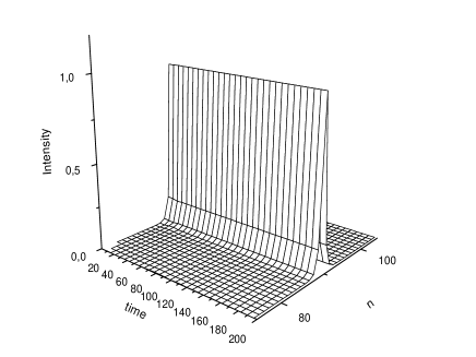
Figure 8: Evolution perturbed of staggered odd mode (b) $\lambda=1,v_{0}=1,\gamma=-1.7,\beta_{c}=0.140<\beta=0.167$.

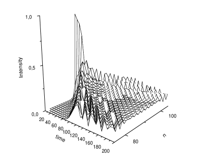
Figure 9: Evolution of perturbed staggered odd mode (b) $\lambda=1,v_{0}=1,\gamma=-1.6,\beta_{c}=0.146>\beta=0.143$.

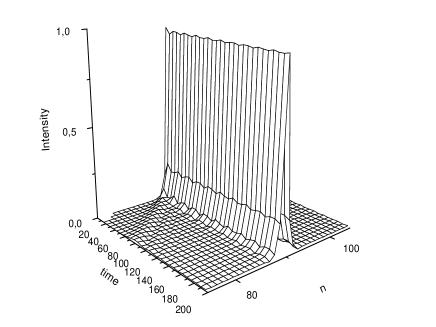
Figure 10: Evolution of perturbed unstaggered odd mode (a) $\lambda=1,v_{0}=1,\gamma=-0.3$.

V Conclusion

In conclusion we have investigated the modulational instabilities and discrete breathers in BEC with two- and three-body interactions in the optical lattice. Following to the procedure suggested in Alfimov we derive the lattice nonlinear model which describe the GP equation with periodic potential. This approximation is reasonable for the atomic wave function is approximated by a single Wannier function - so called a Wannier soliton. The modulational instability in a lattice is the process leading to the generation of discrete breathers in the optical lattice. We find the regions of instabilities of nonlinear plane wave and conform analytical predictions by the direct numerical simulations of the CQDNLS equation. The lattice dispersion vary sign in dependence of the quasi-momentum value in the Brilloin zone. Thus we can control the regions of instability even for the fixed signs of two and three body interactions. This circumstance extend the possibility for creation of the localized modes in BEC in optical potential. We find the expressions for the amplitudes and frequencies of different strongly localized modes in optical lattice such as even, odd, twisted stuggered and unstaggered modes. We analyze the stability of these modes and found the stability regions which are necessary for the search of these modes in the experiments with BEC in optical lattice. For the further investigations will be interesting to consider the regimes beyond of the tight-binding approximation(the deep optical lattice limit) by accounting the higher order terms in the Wannier expansion. In particular it concerns the extensions of CQDNLSE involving the discrete nonlinear models with nonlocal nonlinearitiesTS2 ; Alfimov ; KevPel ; Khare .

References

- (1) S. Flash and C.R. Willis, Phys.Rep. 295, 181 (1998);
- (2) The focus issue on ”Nonlinear localized modes:physics and applications,” Chaos 13, 586 (2003).
- (3) F. Lederer, S. Darmanyan, and A. Kobyakov, in Nonlinearity and Disorder: Theory and Applications, F. Kh. Abdullaev, O. Bang and M. P. Soerensen (Eds.). Kluwer AP, pp.131-157 (2001).
- (4) A. Trombettoni and A. Smerzi, Phys.Rev.Lett. 86, 2353 (2001).
- (5) F.Kh. Abdullaev, B.B. Baizakov, S.A. Darmanyan, V.V. Konotop, and M. Salerno, Phys.Rev. A 64, 043606 (2001).
- (6) V.A. Brazhnyi and V.V. Konotop, Mod.Phys.Lett. B 18, 627 (2004).
- (7) G.Alfimov, P.G. Kevrekidis, V.V. Konotop, and M. Salerno, Phys.Rev. E 66, 046608 (2002).
- (8) P.G. Kevrekidis, D.J. Frantzeskakis, Mod.Phys.Lett. B 18, 173 (2004).
- (9) F.Kh. Abdullaev and V.V. Konotop, Phys.Rev. A 68, (2003).
- (10) Morsh and M. Oberthaler, Rev.Mod.Phys. 78, 179 (2006).
- (11) B.Eiermann, Th. Anker, M. Ablietz, M. Taglieber, P. Treutlein, K.-P. Marzlin, and M.K. Oberthaler, Phys.Rev.Lett. 92, 320401 (2004).
- (12) W. Zheng, E.M. Wright, H. Pu, and P. Meystre, Phys.Rev. A 68, 023605 (2003).
- (13) F.Kh. Abdullaev, A. Gammal, L. Tomio and T. Frederico, Phys.Rev. A 63, 043604 (2001).
- (14) N. Akhmediev, M.P. Das, and A.V. Vagov, Int.J.Mod.Phys. B 13, 625 (1999).
- (15) T. Kraemer et al., arXive:cond-mat/0512394.
- (16) F.Kh. Abdullaev and M. Salerno, Phys.Rev. A 72, 033617 (2005).
- (17) R. Carretero-Gonzales, J.D. Talley, C. Chong, and B.A. Malomed, arXive:nlin/0512052.
- (18) D. Cai, A.R. Bishop, and N. Gronblech-Jensen, Phys.Rev.Lett. 70, 591 (1993).
- (19) F.Kh. Abdullaev, S.A. Darmanyan, and J. Garnier, Progress in Optics, E.Wolf(Ed.), 42, 301 (2002).
- (20) J.B. Page, Phys.Rev. B 41, 7835 (1990).
- (21) S. Darmanyan, A. Kobyakov, and F. Lederer, JETP 86, 682 (1998).
- (22) A. Smerzi and A. Trombettoni, Phys.Rev.A 68, 023613 (2003).
- (23) P.G. Kevrekidis, S.V. Dmitriev, and A.A. Sukhorukov, arXive:nlin/0603046.
- (24) A.Khare, K.Rasmussen, M. Salerno, M. Samuelsen, and A. Saxena, arXive:clin/0603034.