Statistical mechanics of combinatorial auctions

Abstract

Combinatorial auctions are formulated as frustrated lattice gases on sparse random graphs, allowing the determination of the optimal revenue by methods of statistical physics. Transitions between computationally easy and hard regimes are found and interpreted in terms of the geometric structure of the space of solutions. We introduce an iterative algorithm to solve intermediate and large instances, and discuss competing states of optimal revenue and maximal number of satisfied bidders. The algorithm can be generalized to the hard phase and to more sophisticated auction protocols.

Auctions constitute an important part of economic activity Krishna . With today’s pronounced role of e-commerce and the use of the internet as a world-wide market place, fundamental changes have occurred in the use of auctions. Their popularity has increased due to freely accessible web services, and both the range and the nature of objects which can be bought and sold have diversified. Single-item auction protocols are however inappropriate when the number of objects to be sold is large, especially if buyers are interested in bundles of objects with complementary features. In such cases, it is preferrable to allow buyers to bid on combinations of objects instead of single items. Such auctions are referred to as combinatorial auctions (CA). Initially motivated by the problem of airport time slot allocation and by the distribution of radio spectrum licenses, CA are now widely used in a variety of contexts MIT . Finding the maximum auctioneer’s payoff allocation to a given CA is a computationally hard problem requiring exponential time resources. Fast and efficient heuristic algorithms are thus needed to identify optimal or close-to-optimal allocations, and models of CA are here of interest as theoretical benchmarks Sandholm ; vohra .

In this Letter, we will first map a generic CA problem onto a geometrically constrained lattice gas defined on a sparse random graph, coupled to a local chemical potential. This allows us to relate the computational complexity of determining optimal allocations to the glassy behaviour induced by the geometric frustration of the system. The latter here results from conflicting bids. The statistical mechanics approach to Bethe lattice glass models rivoire then allows us to characterize the typical properties of large random instances of CA, and to formulate algorithms for solving single instances.

A simple CA model describes $N$ players and a total set of $M$ items to be sold. Each player $i$ bids for an individual subset $A_{i}\subseteq\{1,\dots,M\}$ for which he is willing to pay a price $\nu_{i}>0$. It is understood here that the player is only interested in the full set $A_{i}$, but not in any proper subset. The bid of player $i$ is thus given by the pair $(A_{i},\nu_{i})$. More complex CA where bidders submit lists of $n_{i}\geq 1$ subset-price pairs, $\{(A_{i}^{\ell},\nu_{i}^{\ell})\}_{l=1,...,n_{i}}$ nested by logical ORs or XORs can be reduced to the case of single-item bids, with a possibly enlarged set of bidders and items Nisan . Hence we shall confine our discussion to the $n_{i}=1$ case of single-subset bids.

Let us indicate a successful bid by $x_{i}=1$, and an unsuccessful one by $x_{i}=0$. Then the winner determination problem (WDP) consists in finding a ‘configuration’ $\mathbf{x}=(x_{1},\dots,x_{N})\in\{0,1\}^{N}$, which maximizes the auctioneer’s revenue $R=\sum_{i}\nu_{i}x_{i}$ and respects the constraint that each item be sold at most once, i.e., that $x_{i}x_{j}=0$ whenever $A_{i}\cap A_{j}\neq 0$ for a pair $i\neq j$. It is also interesting to discuss how far the optimal solution is from a configuration maximizing the number $N_{s}=\sum_{i}x_{i}$ of satisfied bidders. These two tasks are usually conflicting, and can be formulated as a multi-objective optimization problem whose outcome depends on the optimization priority. In particular we will compare results of procedures first maximizing $R$ and then $N_{s}$, and vice versa.

Deciding which bids $(A_{i},\nu_{i})$ are successful ($x_{i}=1$) is a non-trivial optimization problem, because bids can overlap. If $A_{i}\cap A_{j}\neq\emptyset$ for some $i\neq j$, the two bidders $i$ and $j$ cannot simultaneously be successful. Even an agent with a high bid $\nu_{i}$ is not guaranteed to win, as it may be advantageous for the auctioneer to allocate the items contained in $A_{i}$ to a number of other agents having a higher aggregate revenue. Indeed the CA optimal allocation problem is NP-complete, as can be demonstrated by its equivalence to the weighted set packing problem PAP . NP-completeness, however, refers to a worst-case scenario and does not necessarily imply that one cannot find the optimal solution for some large real-life CA problems.

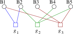
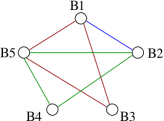
Figure 1: (Color online) Example of a CA interaction network: factor graph (left), and corresponding conflict graph (right). Bidders $B_{i}$ are indicated as circles, items $g_{a}$ as squares attached via links to all the bidders wanting to pay for them. In the conflict graph bidders are connected by a link if and only if they share at least one item. Any item of degree $k$ in the factor graph corresponds to a $k$-clique of vertices in the conflict graph. $I_{a}$ is the set of players bidding for item $a$.

Here, we focus on a simple probabilistic model where each player submits a single bid. This setup retains the same level of computational complexity as more general cases, and the WDP can be reduced to computing the ground state of a lattice gas defined on a suitable random graph, where particles residing on vertices are subject to a geometric constraint as well as to a local chemical potential.

The Model — Let us take $N$ players and $M=\alpha N$ items, with $\alpha={\cal O}(1)$. Player $i$ bids for a subset $A_{i}$ containing $\ell_{i}$ items, and any item $a$ in turn is chosen by $k_{a}$ agents. Any realization of this bidding structure can then be represented by a factor graph containing bidder and item nodes, cf. Fig. 1. A compact representation is given by the conflict graph (CG), in which two players $i$ and $j$ are linked whenever $A_{i}\cap A_{j}\neq\emptyset$. More complex bidding protocols can be cast in the same formalism in-prep .

The CA can be mapped to a lattice gas of particles on the CG, with occupation variables $x_{i}\in\{0,1\}$ representing the bidders’ success/failure. The Hamiltonian ${\cal H}=-R=-\sum_{i}\nu_{i}x_{i}$ describes a coupling of $x_{i}$ to a local field $\nu_{i}$, and it can be associated with a formal inverse temperature $\beta$. A chemical potential $\mu$ allows to control the particle number $N_{s}=\sum_{i}x_{i}$. The grand-canonical partition function of such a lattice-gas reads

$$Z=\sum_{\scriptscriptstyle\mathbf{x}\in\{0,1\}^{N}}\!\!\exp\left(\sum_{i=1}^{N}(\mu+\beta\nu_{i})x_{i}\right)\prod_{(i,j)\in C}(1-{x_{i}x_{j}}),$$ (1)

where $C$ is the set of edges of the CG. The product over $C$ implements the compatibility constraint that each item can be sold at most once, and can be interpreted as a volume exclusion for neighbouring lattice sites. Temperature and chemical potential can be used to select compatible solutions in configuration space: (i) the choice $\beta\to\infty$ and $\mu=0$ corresponds to configurations maximizing $R$ independently of $N_{s}$, (ii) $\beta=0$ and $\mu\to\infty$ selects configurations maximizing $N_{s}$ only, (iii) $\beta\to\infty$ before $\mu\to\infty$: maximizes $N_{s}$ within the subset of configurations of maximal revenue, (iv) $\mu\to\infty$ before $\beta\to\infty$: maximizes $R$ within the subset of compatible configurations of maximum number of satisfied bidders. The maximal revenue can thus be computed as $R^{*}=\lim_{\beta\to\infty}\partial_{\beta}\ln Z$ at finite $\mu$, and the maximum $N_{s}^{*}=\lim_{\mu\to\infty}\partial_{\mu}\ln Z$ at finite $\beta$.

The cavity approach — The search for optimal configurations can be performed efficiently via algorithms based on the cavity method. For a general presentation of the method see e.g. MZ ; book and references therein. Following book , one can introduce cavity biases $\{u_{a\to i}\}$ and cavity fields $\{h_{j\to a}\}$ associated with the links of the factor graph of a single CA instance as illustrated in Fig. 2. The cavity bias $u_{a\to i}$ measures the likelihood that item $a$ is already assigned to another bidder $k\in I_{a}\setminus i$, and cannot be sold to $i$. The cavity field $h_{i\to a}$ is then given by the re-weighted price minus the sum of all $u_{b\to i}$ arriving from $b\in A_{i}$ except from $a$. It measures the likelihood that the bidder would win if his bid did not contain item $a$. The resulting self-consistent equations are the basis of the so-called belief propagation (BP) algorithm:

$$u_{a\to i} = \hat{u}(\{h_{k\to a}\})=\frac{1}{\beta+\mu}\ln\left(1+\sum_{k\in I_{a}\setminus i}e^{(\beta+\mu)h_{k\to a}}\right)$$

$$h_{i\to a} = \hat{h}(\nu_{i},\{u_{b\to i}\})=\frac{\mu+\beta\nu_{i}}{\beta+\mu}-\sum_{b\in A_{i}\setminus a}u_{b\to i}.$$ (2)

If the iteration of Eqs. (2) converges to a fixed point, we can estimate the probability that bid $i$ becomes satisfied:

$$P_{i}\equiv P(x_{i}=1)\simeq\frac{\exp\{(\mu+\beta)H_{i}\}}{1+\exp\{(\mu+\beta)H_{i}\}}$$ (3)

with an effective local field $H_{i}=(\mu+\beta\nu_{i})/(\beta+\mu)-\sum_{b\in A_{i}}u_{b\to i}$. The payoff estimate becomes $\sum_{i}R=\nu_{i}P_{i}$, and the expected number of satisfied bids is $N_{s}=\sum_{i}P_{i}$.

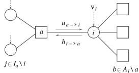
Figure 2: Illustration of cavity biases and fields.

The maximization of these quantities can be achieved by tuning $\beta$ and $\mu$ as described after Eq. (1). In principle, the limit $\beta\to\infty$ at $\mu=0$ – corresponding to a maximum revenue – can be taken directly in Eqs. (2), and has a simple interpretation. In this case $u_{a\to i}$ is a warning to bidder $i$ that he needs to allocate at least a price $u_{a\to i}$ to item $a$ in order to outbid the other players in $I_{a}$. Consequently, in order to secure his subset $A_{i}$, he has to offer at least $\sum_{a\in A_{i}}u_{a\to i}$. The field $H_{i}$ is thus given by the difference between the amount $i$ is willing to pay and the minimal amount required for $i$ to win. If $H_{i}>0$ the bidder will be successful ($x_{i}=1$) with probability $1$ (i.e. in all such solutions), whereas $H_{i}<0$ indicates a loosing bid. Players with $H_{i}=0$ are successful in some optimal assignments, and unsuccessful in others. In order to deal with the latter degeneracy, one has to resort to a more subtle limit of Eqs. (2), allowing for fields vanishing proportionally to the formal temperature.

Eqs. (2) are valid for any fixed choice of the graphs, prices and bids, i.e. the effective fields can be determined for any specific CA instance. They can be solved iteratively in ${\cal O}(N)$ steps whenever the iteration converges. The fields $\{H_{i}\}$ at convergence of the BP iteration can be used as input for an iterative search/decimation procedure, where items are assigned iteratively to bidders with highest $H_{i}$, and BP equations are then iterated for the reduced problem containing only variables not yet fixed in the previous step. This procedure runs in ${\cal O}(N\log N)$ steps if a finite fraction of items is assigned at each step.

Solution for typical cases — To extract analytical estimates for the CA outcomes we average Eqs. (2) over given random factor-graph and price ensembles. In doing so we obtain self-consistent integral equations for the order parameters, i.e. the histograms of both the cavity biases ($Q(u)$) and the cavity fields ($P(h)$). In the so-called replica symmetric (RS) phase MZ ; book , these equations are

$$P(h) = \sum_{\ell=0}^{\infty}\tilde{p}_{\ell}\int\prod_{t=1}^{\ell}du_{t}Q(u_{t})\int d\nu P(\nu|\ell+1)\delta(h-{\hat{h}})$$

$$Q(u) = \sum_{k=1}^{\infty}\tilde{q}_{k}\int\prod_{t=1}^{k}dh_{t}P(h_{t})\delta(u-{\hat{u}})$$ (4)

where $P(\nu|\ell+1)$ is the distribution of prices $\nu$ for agents bidding for sets of $\ell+1$ objects, ${\hat{h}}$, ${\hat{u}}$ are given by (2), $\tilde{p}_{\ell}=(\ell+1)p_{\ell+1}/\langle\ell\rangle$ and $\tilde{q}_{k}=(k+1)q_{k+1}/\langle k\rangle$, where $p_{\ell}$ and $q_{k}$ are the degree distributions of the bidders and items in the factor graph. Eqs. (4) are solved via population dynamics book . Here we focus on two simple non-trivial CA ensembles. In both cases, every player selects each item independently with probability $z/M$. The probability that a player wants $\ell$ items is Poissonian, $p_{\ell}={\rm e}^{-z}z^{\ell}/\ell\,!$, for large $M$. Similarly, the probability that a given item is chosen by $k$ players is $q_{k}={\rm e}^{-\lambda}\lambda^{k}/k\,!$ for large $N$, where $\lambda=z/\alpha$. The considered ensembles differ in the prices the bidders are willing to pay:

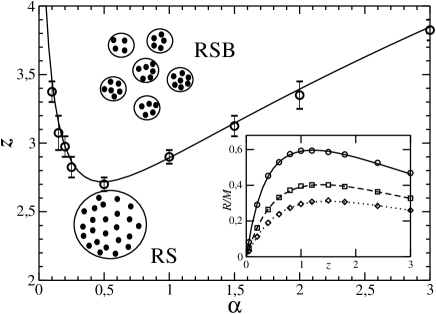
Figure 3: Phase diagram for constant-price CAs in the $(\alpha,z)$-plane: in the lower region, all solutions (maximum-revenue configurations) belong to a single cluster, and RS equations are believed to give the exact revenue result. In the upper region the RS solution is not correct anymore. The symbols mark the point where BP stops to converge on $\sim 3\%$ of the spins ($N=5000$, averaged over $20$ instances), and are consistent with the line at which RS breaks. Inset: Maximal revenue per item vs. $z$ for $\alpha=0.5,1,1.5$ from top to bottom. Average RS results (lines) are compared to simulated-annealing data on single CA instances (markers). Results obtained by iterating BP on the same CA instances (not shown) are consistent with these curves.

(i) Constant prices — Every bidder who bids for at least one object offers the same price $\nu_{i}\equiv 1$. BP-results from Eqs. (4) are shown in the inset of Fig. 3 together with optimal revenue estimates from simulated annealing. Note the maximum of the revenue for intermediate $z$. At small $z$ many items are not element of any bid and do not contribute to the revenue, while at large $z$ items are desired by multiple players resulting in conflicts which restrict the revenue. The main body of the figure shows analytical results in-prep on the validity of RS. Above the phase boundary conflicts induce replica-symmetry breaking (RSB), i.e. a clustering of CA solutions into disconnected sets. RS results cannot be trusted beyond that point and multiple metastable states are found. Note that RSB in the typical case corresponds to non-convergence of BP on relatively large, randomly generated single instances of CAs. This is confirmed by the symbols, which mark the points where BP stops to converge.

(ii) Linear prices — In this second, potentially more realistic case the price of a bid is assumed to equal the size of the desired subset, i.e. the price per item is constant. Qualitatively, the revenue curves show a behaviour similar to the constant-price case, cf. Fig. 4. For small $z$, the revenue is very close to $1-e^{-\lambda}$, the fraction of items wanted by at least one bidder. Even if there is little frustration, it is not possible to sell all items as it would be optimal for the auctioneer in this case note2 . For larger $z$, replica symmetry breaking sets in as a result of increasing frustration, and asymptotically the revenue curves are expected to decrease again with $z$. The increasing level of frustration can also be seen in the fraction of successful players in the group of players placing non-empty bids. As also shown in Fig. 4, this fraction is found to decrease monotonously with $z$, i.e. with the average number of items wanted by a bidder (at fixed $\alpha$).

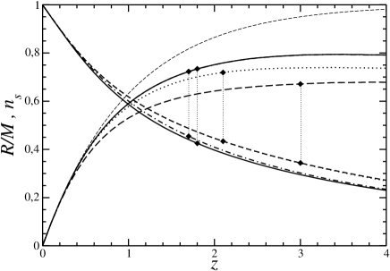
Figure 4: Revenue (increasing curves) and fraction $n_{s}$ of satisfied players in the set of players with non-emtpy bids (decreasing curves) for the four optimization problems ($\alpha=1$). Maximisation order is as follows: (i) $R$ only (full lines), (ii) $N_{s}$ only (dashed lines), (iii) $R$ before $N_{s}$ (dash-dotted lines), (iv) $N_{s}$ before $R$ (dotted lines). Revenues for (i) and (iii) indistiguishable, $n_{s}$ for (ii) and (iv) indistinguishable. Symbols mark the points where RS breaks down, RS results are approximations at large $z$. The upper most increasing line marks the fraction of items which are part of at least one bid, i.e. the theoretical maximum number of auctionable objects.

(iii) Other ensembles— Other CA ensembles give rise to even more complex phase diagrams. For instance, in the elementary case of each player wanting a fixed number $K$ of randomly chosen items, all at the same price (corresponding to $\nu_{i}=const$), one finds that the space of optimal solutions is divided into an exponential number of geometrically distant clusters even for values of $\alpha$ at which all items can be assigned without frustration. This corresponds to a 1-RSB mechanism observed in other hard combinatorial problems book . In such a region (e.g. $\alpha\in[.56,.59]$ for $K=5$) message-passing algorithms MZ ; in-prep provide efficient techniques for finding optimal assignments.

The extension to CAs with generic price distribution is straightforward and will be presented elsewhere in-prep .

Let us finally mention that the case of linear prices allows one to study multi-objective strategies for solving the WDP going beyond standard CA theory which is mostly concerned with revenue maximization. As discussed before, one could also aim to maximize the number of satisfied players. As shown in Fig. 4, doing this after maximizing the revenue has only very little effect on $N_{s}$. On the other hand, maximizing $N_{s}$ independently of the revenue leads to a substantial decrease in $R$. The latter can be partially cured by maximizing the revenue within the set of winner assignments of maximal $N_{s}$, but also there the revenue remains well below its maximum. A suitable strategy of taking into account both $R$ and $N_{s}$ might be to send both $\beta$ and $\mu$ to $\infty$, with a fixed ratio $\beta/\mu$ controling the relative importance of either optimization task. By varying it one can continuously tune the results between the extremes given before.

To conclude, we have presented a statistical physics approach to the CA problem and introduced an iterative algorithm for solving the WDP of large instances of simple CAs. A relatively large body of literature has been devoted to algorithms for solving WDP, such as branch-and-bound and mixed integer programming techniques (see Sandholm ; vohra and references therein). It would be interesting to compare the performance of message-passing algorithms with the existing approaches to WDP, as it has been done recently for satisfiability problems in Refs. erik ; mikko .

This work was supported by the EC Human Potential Programme, contracts HPRN-CT-2002-00319, STIPCO, EU NEST No. 516446, COMPLEXMARKETS and EU IP No. 1935, EVERGROW.

References

- (1) V. Krishna, Auction Theory (Academic Press, 2002).
- (2) P. Cramton, Y. Shoham and R. Steinberg eds., Combinatorial Auctions, (MIT Press, 2006)
- (3) T. Sandholm, in ref. MIT , and Artificial Intelligence 135, 1 (2002)
- (4) S. de Vries and R. Vohra, INFORMS J. of Computing 15, 284 (2003)
- (5) O. Rivoire, O. Martin, G. Biroli and M. Mézard, Eur. Phys. J. B 37, 55 (2004); H. Hansen-Goos and M. Weigt, J. Stat. Mech. P04006 (2006); and references therein.
- (6) N. Nisan, in ref. MIT .
- (7) C. H. Papadimitriou, Computational Complexity, (Addison Wesley Longman, 1995).
- (8) A. Hartmann and M. Weigt, Phase Transitions in Combinatorial Optimization Problems, (Wiley, 2005).
- (9) M. Mézard, G. Parisi, and R. Zecchina, Science 297, 812 (2002); M. Mézard and R. Zecchina, Phys. Rev. E 66, 056126 (2002)
- (10) T. Galla et al., in preparation.
- (11) If each item is wanted by at least two players, a maximally satisfiable phase may exist in-prep .
- (12) E. Aurell, U. Gordon and S. Kirkpatrick, Adv. Neural Inform. Process. Syst. 17, 49 (2005)
- (13) S. Seitz, M. Alava and P. Orponen, J. Stat. Mech. P06006 (2005)