Time Quantified Monte Carlo Algorithm for Interacting Spin Array Micromagnetic Dynamics

Abstract

In this paper, we reexamine the validity of using time quantified Monte Carlo (TQMC) method [Phys. Rev. Lett. 84, 163 (2000); Phys. Rev. Lett. 96, 067208 (2006)] in simulating the stochastic dynamics of interacting magnetic nanoparticles. The Fokker-Planck coefficients corresponding to both TQMC and Langevin dynamical equation (Landau-Lifshitz-Gilbert, LLG) are derived and compared in the presence of interparticle interactions. The time quantification factor is obtained and justified. Numerical verification is shown by using TQMC and Langevin methods in analyzing spin-wave dispersion in a linear array of magnetic nanoparticles.

I Introduction

The TQMC method is found to be a powerful simulation technique in modeling magnetization reversal dynamics of magnetic nanoparticles Nowak et al. (2000); Hinzke and Nowak (2000); Chubykalo et al. (2003a); Cheng et al. (2005, 2006). It is found that simulation with the TQMC method is considerably more efficient than the conventional method of modeling magnetization dynamics based on time-step integration of the stochastic LLG equation, especially in the case of high damping limits Chubykalo et al. (2003a). The attraction of TQMC also lies on the fact that it establishes an analytical connection between the two stochastic simulation schemes, Monte Carlo (MC) and Langevin dynamics, which were previously thought to have different theoretical bases. Such analytical connection provides alternative techniques to both stochastic models, e.g. solving a stochastic differential equation using advanced Monte Carlo techniques to calculate the long-time reversal Cheng et al. (2005); Chubykalo-Fresenko and Chantrell (2005).

The validity of using TQMC to simulate an isolated single domain particle is first demonstrated by Nowak et al. Nowak et al. (2000) and later rigorously proved by us in Ref. Cheng et al. (2006) using the Fokker-Planck equation as a bridge between MC and Langevin methods. In the case of interacting spin arrays, the validity of TQMC has not been analytically proved although it has been numerically shown Hinzke and Nowak (2000); Cheng et al. (2006). It thus comes the necessity to establish the proof for the case of interacting spin systems, since in practical applications the discrete spins or moments (in the form of magnetic nanoparticles) are usually closely packed together, and hence are strongly coupled to one another. It is also important to show explicitly whether the analytical equivalence between the TQMC and the stochastic LLG equation and the time quantification factor, are dependent in any way on the nature (e.g. magnetostatic or exchange) or strength of the coupling interactions.

In this paper, we provide a rigorous proof for this case, based on the technique presented in our earlier works Cheng et al. (2006). We further demonstrate the generality of the TQMC method, by implementing it in two different contexts, i.e. in time-evolution and reversal studies of a square array of spins, and in analyzing the spin wave dispersion in a linear spin chain.

II Model

The physical model under consideration is a spin array (which represent an array of magnetic nanoparticles), whose spin configuration is represented as $\{\mathbf{s}\}=\{\cdots,\hat{\mathbf{s}}_{i},\cdots\}$, where $\mathbf{s}=\mathbf{M}/M_{s}$ is a normalized unit vector representing the magnetic moment of the spin and $i$ refers to the $i^{\mathrm{th}}$ spin in the vector list of length $N$.

The micromagnetic dynamics of the spin array is traditionally described by the Landau-Lifshitz-Gilbert (LLG) equation:

$$\frac{d}{dt}\{\mathbf{s}\}=-\frac{\gamma_{0}H_{k}}{1+\alpha^{2}}\{\mathbf{s}\}\times\left(\{\mathbf{h}\}+\alpha\cdot\{\mathbf{s}\}\times\{\mathbf{h}\}\right)$$ (1)

where $\alpha$ and $\gamma_{0}$ are the damping constant and the gyromagnetic constant respectively, $\{\mathbf{h}\}=\frac{1}{2K_{u}V}\nabla_{\{\mathbf{s}\}}E$ is the effective field which is normalized with respect to the anisotropy field $H_{k}=2K_{u}/\mu_{0}M_{s}$, where $K_{u}$ is the anisotropy constant and $\mu_{0}$ is the magnetic permeability. $E=E(\{\mathbf{s}\})$ is the total energy of the system which consists of the typical contributions in a micromagnetic system, e.g., Zeeman term, anisotropy term, magnetostatic term and exchange coupling term. The operator $\{\mathbf{s}\}\times\{\mathbf{h}\}=\{\cdots,\mathbf{s}_{i}\times\mathbf{h}_{i},\cdots\}$ is understood. To represent the thermal fluctuation, white noise-like stochastic thermal fields are added to the effective field according to Brown Brown (1963).

Alternatively, Random walk Monte Carlo (MC) algorithm can also be used in simulating the magnetization reversal dynamics Nowak et al. (2000). At each Monte Carlo step, one of the $N$ spin sites is randomly selected to undergo a trial move, in which a random displacement lying within a sphere of radius $R$ ($R\ll 1$) is added into the original magnetic moment and the resulting vector is then renormalized. The magnetic moment changes according to a heat bath acceptance rate as $A(\Delta E)=1/(1+\exp(\beta\Delta E))$. Here $\Delta E$ is the energy change within the random walk step and $\beta=(k_{B}T)^{-1}$, $k_{B}$ is the Boltzmann constant and $T$ is the temperature in Kelvin.

III Fokker-Planck Equations

To link the MC scheme with the stochastic LLG equation, we shall derive the respective Fokker-Planck (FP) coefficients corresponding to the LLG equation and the random walk MC Cheng et al. (2006). The general Fokker-Planck equation (FPE) for a spin array in a spherical coordinates is given as

$$\frac{d}{dt}P(\{\theta\},\{\varphi\},t) = -\sum_{i}\frac{\partial}{\partial\theta_{i}}\left(A_{\theta_{i}}\cdot P\right)-\sum_{i}\frac{\partial}{\partial\varphi_{i}}\left(A_{\varphi_{i}}\cdot P\right)+\frac{1}{2}\sum_{i,j}\frac{\partial^{2}}{\partial\theta_{i}\partial\theta_{j}}\left(B_{\theta_{i}\theta_{j}}\cdot P\right)$$ (2)

$$+\frac{1}{2}\sum_{i,j}\frac{\partial^{2}}{\partial\varphi_{i}\partial\varphi_{j}}\left(B_{\varphi_{i}\varphi_{j}}\cdot P\right)+\frac{1}{2}\sum_{i,j}\frac{\partial^{2}}{\partial\theta_{i}\partial\varphi_{j}}\left((B_{\theta_{i}\varphi_{j}}+B_{\varphi_{j}\theta_{i}})\cdot P\right)$$

where drift terms $A_{x}$ and diffusion terms $B_{xy}$ ($x=\{\theta_{i},\varphi_{i}\}$, $y=\{\theta_{j},\varphi_{j}\}$) are defined as the ensemble mean of an infinitesimal change of $x$ and $y$ with respect to time Risken (1967). By giving the detailed derivation in the appendix, we obtained the Fokker-Planck coefficients for LLG:

$$A^{LLG}_{\theta_{i}} = -h^{\prime}\frac{\partial E}{\partial\theta_{i}}-g^{\prime}\frac{1}{\sin\theta_{i}}\frac{\partial E}{\partial\varphi_{i}}+k^{\prime}\cot\theta_{i}$$

$$A^{LLG}_{\varphi_{i}} = g^{\prime}\frac{1}{\sin\theta_{i}}\frac{\partial E}{\partial\theta_{i}}-h^{\prime}\frac{1}{\sin^{2}\theta_{i}}\frac{\partial E}{\partial\varphi_{i}}$$

$$B^{LLG}_{\theta_{i}\theta_{j}} = 2k^{\prime}\cdot\delta_{ij}$$ (3)

$$B^{LLG}_{\varphi_{i}\varphi_{j}} = \frac{1}{\sin^{2}\theta_{i}}2k^{\prime}\cdot\delta_{ij}$$

$$B^{LLG}_{\theta_{i}\varphi_{j}} = B^{LLG}_{\varphi_{j}\theta_{i}}=0$$

as well as for the TQMC:

$$A_{\theta_{i}}^{MC} = N^{-1}\frac{R^{2}}{20}\left(\cot\theta_{i}-\beta\frac{\partial E}{\partial\theta_{i}}\right)$$

$$A_{\varphi_{i}}^{MC} = -N^{-1}\frac{1}{\sin^{2}\theta_{i}}\frac{R^{2}}{20}\beta\frac{\partial E}{\partial\varphi_{i}}$$

$$B_{\theta_{i}\theta_{j}}^{MC} = N^{-1}\frac{R^{2}}{10}\cdot\delta_{ij}$$ (4)

$$B_{\varphi_{i}\varphi_{j}}^{MC} = N^{-1}\frac{1}{\sin^{2}\theta_{i}}\frac{R^{2}}{10}\cdot\delta_{ij}$$

$$B_{\theta_{i}\varphi_{j}}^{MC} = B_{\varphi_{j}\theta_{i}}^{MC}=0$$

where in Eq. (III), $h^{\prime}=\frac{\alpha\gamma_{0}}{\mu_{0}VM_{s}(1+\alpha^{2})}$, $g^{\prime}=h^{\prime}/\alpha$, $k^{\prime}=h^{\prime}/\beta$.

IV Mapping MC to LLG

In the high damping limit where the damping constant $\alpha$ is large, so that $g^{\prime}=h^{\prime}/\alpha\to 0$, a term-wise equivalence can be established between the FPE coefficients in Eqs. (III) and (III), corresponding to the LLG and MC methods, if:

$$R^{2}\Delta\tau_{\mathrm{\scriptscriptstyle MC}}=\frac{20\alpha}{1+\alpha^{2}}\frac{\gamma_{0}}{\beta\mu_{0}VM_{s}}\Delta t_{\mathrm{\scriptscriptstyle LLG}}.$$ (5)

Eq. (5), in which $\Delta\tau_{\mathrm{\scriptscriptstyle MC}}$ is calibrated in MCS/site (one Monte Carlo step for each site on the average), is the time quantification factor for the TQMC method in interacting spin arrays. The time quantification factor is found to be the same as the one in Ref. Nowak et al. (2000) for an isolated single particle case, and is thus consistent with previous numerical convergence observed in Refs. Hinzke and Nowak (2000); Cheng et al. (2006).

For the low damping limit where precessional motion becomes significant, one may wish to use the precessional (hybrid) Metropolis Monte Carlo algorithm Cheng et al. (2006). We confirm that, by using the same derivation techniques, one is able to prove the validity of including the precessional move in the MC algorithm in simulating the micromagnetic properties of an interacting spin array.

V Results and Discussion

The equivalence between the MC method and LLG, which is expressed by Eq. (5), provides the theoretical justification for the use of MC method as an alternative to the LLG equation in micromagnetic studies. The equivalence which has been established is very general because no explicit form of the Hamiltonian is used in the derivation. This implies that the validity of the equivalence is independent of many physical and simulation parameters. For illustration, we test the validity of the TQMC method for a simple $10\times 10$ spin array which is subject to a varying exchange coupling strength $J$. As shown in Fig. (1), the time evolution behavior of the (asymmetric) magnetization reversal is simulated for different values of $J$. We find good convergence between the simulated results from both LLG and MC schemes, even when the switching mechanism of the spin array changes from the independent reversal (small $J$) to the nucleation-driven reversal (large $J$). We also confirm that the mapping between MC and LLG time steps as expressed in Eq. (5), is also independent of other simulation and physical parameters, e.g. the chosen boundary condition (periodic / free), the lattice size, and the nature of the coupling (magnetostatic / exchange).

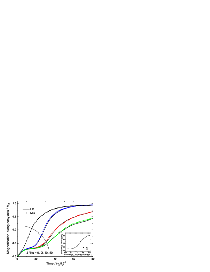
Figure 1: (color online) The time evolution behavior of the magnetization reversal in a spin array system. The following simulation parameters are assumed: lattice size of $10\times 10$, periodical boundary condition, thermal condition $K_{u}V/k_{B}T=25$, damping constant $\alpha=1.0$ and external field $h=0.5$ applied on an angle $\theta=\pi/4$ with respect to the easy axes. The exchange coupling strength $J$ is the adjustable variable. To guarantee the simulation accuracy, the time interval $\Delta t$ for the LLG integration changes with $J$ as $\Delta t=0.01/(1+h+J/K_{u}V)$ Dimitrov and Wysin (1994), while the trial move step size $R$ in the MC simulation is chosen to reflect the $\Delta t$ in one MCS. Error bars are smaller than the symbol size.

Next, we show that the equivalence between the MC method and LLG enables the MC method to be utilized in most of the situations where LLG applies, and beyond the above time-evolution simulation. As an example, we consider the dispersion relation for the primary spin wave mode of a one-dimensional spin chain. This example is chosen because it tests the capability of precessional TQMC method to simulate both spatial and time correlation of the spin-wave dynamics. By comparison, conventional MC methods are more suited for equilibrium or steady-state studies rather than time correlation dynamics.

The Hamiltonian of the spin chain system is set to be:

$$\mathcal{H}=\sum_{i}\left(-J\sum^{\{i\}}_{j<i}\hat{\mathbf{s}}_{i}\cdot\hat{\mathbf{s}}_{j}-K_{u}V(\hat{\mathbf{s}}_{i}\cdot\hat{\mathbf{k}}_{n})^{2}-\mu_{0}M_{s}V\cdot\hat{\mathbf{s}}_{i}\cdot\mathbf{H}_{\mathrm{ext}}\right)$$ (6)

where $\{i\}$ represents the neighboring spins of the $i^{\mathrm{th}}$ spin, $J$ is the coupling strength, $\mathbf{H}_{\mathrm{ext}}$ is the applied field and $\hat{\mathbf{k}}_{n}$ refers to the unit vector along the easy axis. Magnetostatic coupling was not included in this test. The dispersion relation for the one-dimensional spin wave mode has been theoretically studied Kittel (1996) and is given by:

$$\omega(k)=\frac{\gamma_{0}H_{k}}{1+\alpha^{2}}[1+h_{\mathrm{ext}}+4(J/2K_{u}V)\sin^{2}(ka/2)]$$ (7)

where $h_{\mathrm{ext}}=H_{\mathrm{ext}}/H_{k}$ and $a$ is the lattice constant. The calculations were done using the computational techniques of Refs. Chantrell et al. (1998); Chubykalo et al. (2002). Spins were initially aligned along the $z$ direction, in parallel with both the easy axes and applied fields. Stochastic simulation was performed on this initial configuration for 100 $(\gamma_{0}H_{k})^{-1}$, in order to achieve the quasi-equilibrium state. Space and time Fourier transforms were then performed on the off-axis components. From the resulting spin wave spectra, the peak frequency $\omega$ determined for a range of wavevector $k$. The resulting dispersion relation in Fig. (2) shows a very good convergence between the simulated results (calculated from both LLG and MC) and the theoretical prediction of Eq. (7).

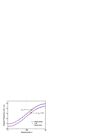
Figure 2: (color online) Dispersion relation for the simulated spin wave mode. Simulation parameters are: chain length $N=200$, free boundary condition, thermal condition $K_{u}V/k_{B}T=50$, exchange coupling strength $J/2K_{u}V=1$ and damping constant $\alpha=0.1$. Kittel’s model refers to the theoretical dispersion relation of Eq. (7).

However, there do exist limitations to the TQMC method. The TQMC method cannot be easily extended for some advanced micromagnetic simulations, which include e.g. the spin torque effect, as compared to the stochastic LLG model. In addition, even though we found the TQMC algorithm to be typically 2–5 times faster than the LLG-based simulation with an equivalent time step, it is still too inefficient to model long-time magnetization reversal of up to, say, 1 second. Nevertheless, our analysis has raised the possibility of developing advanced time-quanti able Monte Carlo methods, based on e.g. the N-fold way Monte Carlo algorithm Novotny (1995) and kinetic Monte Carlo method Chubykalo-Fresenko and Chantrell (2005), for micromagnetic studies.

VI Conclusion

We have derived the time quantification factor which relate the time-scales of TQMC method and Langevin dynamics in the stochastic simulation of an interacting array of nanoparticles. The time quantification factor is found to be the same as that derived previously for isolated single-domain particles, up to the linear-order in the time-step size $\Delta t$. No explicit form of the Hamiltonian is implied in the derivation, which means that the equivalence between the two stochastic schemes is general and independent of many physical and simulation parameters. To demonstrate this, we implement the TQMC scheme for the study of i) time evolution and magnetization reversal in a square spin array, and ii) spin wave behavior in a one-dimensional interacting array of particles. In the case of (i), we show a close correspondence between the TQMC and LLG results for a wide range of coupling strength. The equivalence remains valid even when the reversal mode changes as $J$ is increased. In the case of (ii), the numerical verification of the time quantification factor is provided by the close agreement of the spin wave dispersion curves as obtained by both TQMC and Langevin dynamical methods. The two curves also show a very close agreement to the known theoretical dispersion relation. Our analytical derivation and numerical studies thus justify the applicability of the TQMC method for stochastic micromagnetic studies in most cases where the LLG equation applies.

VII Appendix

VII.1 FP coefficients for the LLG equation

A previous study of the effect of thermal fluctuations in an interacting spin array system based on the Langevin scheme, showed that the inter-particle interactions do not result in any correlations of the thermal fluctuations Chubykalo et al. (2003b). However, to the best of our knowledge, a detailed derivation of the FP coeffcients for an interacting particle system has not been presented. Hence we include, as an appendix, a derivation of FP coefficients for an interacting particle system. We extend Brown’s derivation Brown (1963) for the FP coefficients of isolated single domain particles to obtain the FP coefficients for the case of interacting particles.

The thermal field $\mathbf{h}(t)$ representing the thermal fluctuations, according to Brown Brown (1963), has the properties of a white noise, i.e.

$$\left<h_{i}^{p}(t)\right>=0,\quad\left<h_{i}^{p}(0)h_{j}^{q}(t)\right>=2D\cdot\delta_{pq}\delta_{ij}\delta(t)$$ (8)

where $i,j=\{1,2,3\}$ denote the Cartesian coordinates component $\{x,y,z\}$ and $p,q=\{1,\ldots,N\}$ refer to the $p^{\mathrm{th}}$ and $q^{\mathrm{th}}$ spin in the list. Hence, if:

$$K_{i}^{p}\equiv\int_{t}^{t+\Delta t}h_{i}^{p}(t^{\prime})dt^{\prime}$$ (9)

then

$$\left<K_{i}^{p}\right>=0,\quad\left<K_{i}^{p}K_{j}^{q}\right>=2D\cdot\delta_{pq}\delta_{ij}\Delta t$$ (10)

Rewriting Eq. (1) in spherical coordinates, we obtain

Left side $$= \frac{d\mathbf{s}_{i}}{dt}=\frac{\partial\mathbf{s}_{i}}{\partial\theta_{i}}\frac{d\theta_{i}}{dt}+\frac{\partial\mathbf{s}_{i}}{\partial\varphi_{i}}\frac{d\varphi_{i}}{dt}=\vec{\mathbf{e}}_{\theta}\cdot\dot{\theta}_{i}+\vec{\mathbf{e}}_{\varphi}\cdot\sin\theta_{i}\dot{\varphi}_{i}$$ (11)

Right side $$= \frac{\gamma_{0}}{\mu_{0}M_{s}V(1+\alpha^{2})}\left(\mathbf{s}_{i}\times\frac{\partial E}{\partial\mathbf{s}_{i}}+\alpha\cdot\mathbf{s}_{i}\times\left(\mathbf{s}_{i}\times\frac{\partial E}{\partial\mathbf{s}_{i}}\right)\right)$$ (12)

$$= \left(-h^{\prime}\frac{\partial E}{\partial\theta_{i}}-g^{\prime}\frac{1}{\sin\theta_{i}}\frac{\partial E}{\partial\varphi_{i}}\right)\vec{\mathbf{e}}_{\theta}+\left(g^{\prime}\frac{\partial E}{\partial\theta_{i}}-h^{\prime}\frac{1}{\sin\theta_{i}}\frac{\partial E}{\partial\varphi_{i}}\right)\vec{\mathbf{e}}_{\varphi}$$

in which the partial differential relationships such as $\frac{\partial E}{\partial\mathbf{s}}=\frac{\partial E}{\partial\theta}\frac{\partial\theta}{\partial\mathbf{s}}+\frac{\partial E}{\partial\varphi}\frac{\partial\varphi}{\partial\mathbf{s}}=\frac{\partial E}{\partial\theta}\vec{\mathbf{e}}_{\theta}+\frac{\partial E}{\partial\varphi}\frac{1}{\sin\theta}\vec{\mathbf{e}}_{\varphi}$ have been used. With the inclusion of the thermal fluctuation, additional terms will be added into the right side as $-\frac{\gamma_{0}H_{k}}{1+\alpha^{2}}\left(\mathbf{s}_{i}\times\mathbf{h}(t)+\alpha\cdot\mathbf{s}_{i}\times\left(\mathbf{s}_{i}\times\mathbf{h}(t)\right)\right)$. By considering the relation between Cartesian and spherical base vectors:

$$\vec{\bm{i}} = \sin\theta\cos\varphi\cdot\vec{\mathbf{e}}_{r}+\cos\theta\cos\varphi\cdot\vec{\mathbf{e}}_{\theta}-\sin\varphi\cdot\vec{\mathbf{e}}_{\varphi}$$

$$\vec{\bm{j}} = \sin\theta\sin\varphi\cdot\vec{\mathbf{e}}_{r}+\cos\theta\sin\varphi\cdot\vec{\mathbf{e}}_{\theta}+\cos\varphi\cdot\vec{\mathbf{e}}_{\varphi}$$

$$\vec{\bm{k}} = \cos\theta\cdot\vec{\mathbf{e}}_{r}-\sin\theta\cdot\vec{\mathbf{e}}_{\theta}$$ (13)

and equating Eqs. (11) and (12), we thus obtain $2N$ simultaneous equations as:

$$\frac{d\theta_{i}}{dt} = h^{\prime}H_{\theta_{i}}^{\prime}+g^{\prime}\frac{1}{\sin\theta_{i}}H_{\varphi_{i}}^{\prime}$$

$$\frac{d\varphi_{i}}{dt} = -g^{\prime}\frac{1}{{\sin\theta_{i}}}H_{\theta_{i}}^{\prime}+h^{\prime}\frac{1}{{\sin^{2}\theta_{i}}}H_{\varphi_{i}}^{\prime}$$ (14)

where

$$H_{\theta_{i}}^{\prime}=-\frac{\partial E}{\partial\theta_{i}}+H_{\theta_{i}},\quad H_{\varphi_{i}}^{\prime}=-\frac{\partial E}{\partial\varphi_{i}}+H_{\varphi_{i}}$$ (15)

$H_{\theta_{i}}$ and $H_{\varphi_{i}}$ are the contributions of $\mathbf{h}(t)$ to the generalized forces corresponding to $\theta_{i}$ and $\varphi_{i}$ :

$$(2K_{u}V)^{-1}H_{\theta_{i}} = h_{1}^{i}(t)\cos\theta_{i}\cos\varphi_{i}+h_{2}^{i}(t)\cos\theta_{i}\sin\varphi_{i}-h_{3}^{i}(t)\sin\theta_{i}$$

$$(2K_{u}V)^{-1}H_{\varphi_{i}} = -h_{1}^{i}(t)\sin\theta_{i}\sin\varphi_{i}+h_{2}^{i}(t)\sin\theta_{i}\cos\varphi_{i}$$ (16)

Eq. (14) can be expressed directly in a general form as:

$$\dot{x}_{i}^{p}=F_{i}^{p}(x)+\sum_{k=1}^{3}{G_{ik}^{p}(x)h_{k}^{p}(t)}$$ (17)

where $x$ represents the set of $2N$ variable $\{x_{i}^{p}\}$ (here $i=\{1,2\}$ denotes angular coordinates $\{\theta,\varphi\}$ and $p=\{1,2,\ldots,N\}$ refers to the $p^{\mathrm{th}}$ spin in the list). To evaluate the FP coefficients $A_{x_{i}}$ and $B_{x_{i}x_{j}}$, we need $\Delta x_{i}$ only to terms of the order $\Delta t$ for $A_{x_{i}}$ and only to terms of order $(\Delta t)^{1/2}$ for $B_{x_{i}x_{j}}$. Taking note of Eq. (9), $\Delta x_{i}$ itself is of order $(\Delta t)^{1/2}$. Expanding $F_{i}^{p}(x)$ and $G_{ik}^{p}(x)$ in Taylor’s series at initial state $x_{0}$:

$$F_{i}^{p}(x) = F_{i}^{p}(x_{0})+\sum_{q,j}F_{i,j}^{p,q}\cdot\Delta x_{j}^{q}+\frac{1}{2}\sum_{q,r,j,l}F_{i,jl}^{p,qr}\cdot\Delta x_{j}^{q}\Delta x_{l}^{r}+\cdots$$

$$G_{ik}^{p}(x) = G_{ik}^{p}(x_{0})+\sum_{q,j}G_{ik,j}^{p,q}\cdot\Delta x_{j}^{q}+\frac{1}{2}\sum_{q,r,j,l}G_{ik,jl}^{p,qr}\cdot\Delta x_{j}^{q}\Delta x_{l}^{r}+\cdots$$ (18)

where, for example, $F_{i,j}^{p,q}=\partial F_{i}^{p}/\partial x_{j}^{q}$ and $G_{ik,j}^{p,q}=\partial G_{ik}^{p}/\partial x_{j}^{q}$. Hence by integration of Eq. (17) with respect to $\Delta t$, and truncate the terms that has order higher than $\Delta t$, we have:

$$\Delta x_{i}^{p}=F_{i}^{p}\Delta t+\sum_{k}{G_{ik}^{p}}\int_{0}^{\Delta t}{h_{k}^{p}(t_{1})dt_{1}}+\sum_{q,j,k}{G_{ik,j}^{p,q}\int_{0}^{\Delta t}{\Delta x_{j}^{q}h_{k}^{p}(t_{1})dt_{1}}}$$ (19)

and in the last integral we may express $\Delta x_{j}^{q}$ to the order of $\Delta t^{1/2}$, namely, as $\sum_{j}G_{jl}^{q}\int_{0}^{\Delta t_{1}}h_{l}^{q}(t_{2})dt_{2}$. Thus,

$$\Delta x_{i}^{p}=F_{i}^{p}\Delta t+\sum_{k}{G_{ik}^{p}}\int_{0}^{\Delta t}{h_{k}^{p}(t_{1})dt_{1}}+\sum_{q,j,k,l}{G_{ik,j}^{p,q}G_{jl}^{q}\int_{0}^{\Delta t}dt_{1}\int_{0}^{t_{1}}{h_{k}^{p}(t_{1})h_{l}^{q}(t_{2})dt_{2}}}$$ (20)

the second term is of order $\Delta t^{1/2}$, the others of order $\Delta t$; therefore, to the first order in $\Delta t$:

$$\Delta x_{i}^{p}\Delta x_{j}^{q}=\sum_{k,l}{G_{ik}^{p}G_{jl}^{q}\int_{0}^{\Delta t}dt_{1}\int_{0}^{\Delta t}{h_{k}^{p}(t_{1})h_{l}^{q}(t_{2})dt_{2}}}$$ (21)

It is easily seen that the double integral in Eq. (20) is half that in Eq. (21). We now evaluate the statistical average by considering Eq. (10) and dividing by $\Delta t$:

$$A_{x_{i}^{p}} = \lim_{\Delta t\to 0}\frac{\left<\Delta x_{i}^{p}\right>}{\Delta t}=F_{i}^{p}+D\cdot\sum_{k}{G_{ik,j}^{p,p}G_{jk}^{p}}$$

$$B_{x_{i}^{p}x_{j}^{q}} = \lim_{\Delta t\to 0}\frac{\left<\Delta x_{i}^{p}\Delta x_{j}^{q}\right>}{\Delta t}=2D\cdot\sum_{k}G_{ik}^{p}G_{jk}^{p}\cdot\delta_{pq}\delta_{ij}$$ (22)

In the present application,

$$F_{1}^{p} = -h^{\prime}\frac{\partial E}{\partial\theta_{p}}-g^{\prime}\frac{1}{\sin\theta_{p}}\frac{\partial E}{\partial\varphi_{p}}$$

$$F_{2}^{p} = g^{\prime}\frac{1}{\sin\theta_{p}}\frac{\partial E}{\partial\theta_{p}}-h^{\prime}\frac{1}{\sin^{2}\theta_{p}}\frac{\partial E}{\partial\varphi_{p}}$$ (23)

and

$$(2K_{u}V)^{-1}G_{11}^{p} = h^{\prime}\cos\theta_{p}\cos\varphi_{p}-g^{\prime}\sin\varphi_{p}$$

$$(2K_{u}V)^{-1}G_{12}^{p} = h^{\prime}\cos\theta_{p}\sin\varphi_{p}+g^{\prime}\cos\varphi_{p}$$

$$(2K_{u}V)^{-1}G_{13}^{p} = -h^{\prime}\sin\theta_{p}$$ (24)

$$(2K_{u}V)^{-1}G_{21}^{p} = -g^{\prime}\cot\theta_{p}\cos\varphi_{p}-h^{\prime}\csc\theta_{p}\sin\varphi_{p}$$

$$(2K_{u}V)^{-1}G_{22}^{p} = -g^{\prime}\cot\theta_{p}\sin\varphi_{p}+h^{\prime}\csc\theta_{p}\cos\varphi_{p}$$

$$(2K_{u}V)^{-1}G_{23}^{p} = g^{\prime}$$

Partial differentiation of Eqs. (VII.1) with respect to $\theta_{p}$ and $\varphi_{p}$ gives the formulas for the twelve quantities $G_{ik,j}^{p,p}$ $(i,j=1,2;k=1,2,3)$. Substitution of the values of $F_{i}^{p}$, $G_{ik}^{p}$ and $G_{ik,j}^{p,p}$ into Eqs. (22) gives the value of FP coefficients for LLG dynamical equation as follows:

$$A^{LLG}_{\theta_{i}} = -h^{\prime}\frac{\partial E}{\partial\theta_{i}}-g^{\prime}\frac{1}{\sin\theta_{i}}\frac{\partial E}{\partial\varphi_{i}}+k^{\prime}\cot\theta_{i}$$

$$A^{LLG}_{\varphi_{i}} = g^{\prime}\frac{1}{\sin\theta_{i}}\frac{\partial E}{\partial\theta_{i}}-h^{\prime}\frac{1}{\sin^{2}\theta_{i}}\frac{\partial E}{\partial\varphi_{i}}$$

$$B^{LLG}_{\theta_{i}\theta_{j}} = 2k^{\prime}\cdot\delta_{ij}$$ (25)

$$B^{LLG}_{\varphi_{i}\varphi_{j}} = \frac{1}{\sin^{2}\theta_{i}}2k^{\prime}\cdot\delta_{ij}$$

$$B^{LLG}_{\theta_{i}\varphi_{j}} = B^{LLG}_{\varphi_{j}\theta_{i}}=0$$

where $k^{\prime}=D(h^{\prime 2}+g^{\prime 2})(2K_{u}V)^{2}$ is to be determined since the value of $D$ is still unknown. Substituting Eqs. (VII.1) into Eq. (2) and taking note that $P(\{\theta\},\{\varphi\},t)$ should reduce to the Boltzmann distribution at statistical equilibrium $(\partial P/\partial t=0)$, one thus obtain the value of $k^{\prime}$: $k^{\prime}=h^{\prime}/\beta$.

VII.2 FP coefficients for TQMC

We next derive the FP Coefficients for TQMC. The Monte Carlo algorithm starts with a random selection of the spin site. We consider the $i^{\mathrm{th}}$ spin in the list. For a trial move with the displacement vector to be of size $r_{i}$ $(r_{i}<R)$ and angle $\alpha_{i}$ with respect to $\vec{\mathbf{e}}_{\theta}$, we have the corresponding change with respect to $\theta_{i}$ and $\varphi_{i}$ as Cheng et al. (2006)

$$\Delta\theta_{i} = -r_{i}\cos\alpha_{i}+\frac{r_{i}^{2}}{2}\cot\theta_{i}\sin^{2}\alpha_{i}+O\left(r_{i}^{3}\right)$$

$$\Delta\varphi_{i} = r_{i}\frac{1}{\sin\theta_{i}}\sin\alpha_{i}+r_{i}^{2}\frac{\cot\theta_{i}}{\sin\theta_{i}}\cos\alpha_{i}\sin\alpha_{i}+O\left(r_{i}^{3}\right)$$ (26)

The displacement probability of the size to be $r_{i}$ is given by Nowak et al. Nowak et al. (2000) as

$$p(r_{i})=3\sqrt{R^{2}-r_{i}^{2}}/2\pi R^{3}$$ (27)

and the acceptance probability for this trial move is given by the heat bath rate as

$$A\left(\Delta E\right) = \frac{1}{1+\exp\left(\beta\Delta E\right)}$$ (28)

$$\approx \frac{1}{2}\left(1-\frac{1}{2}\beta\left(\frac{\partial E}{\partial\theta_{i}}\Delta\theta_{i}+\frac{\partial E}{\partial\varphi_{i}}\Delta\varphi_{i}\right)\right)$$

where $\Delta E$ is the energy change in the random walk step and $\beta=(k_{B}T)^{-1}$. Integrating over the projected surfaces [see Fig. (1) in Ref. Cheng et al. (2006) for a clear diagram], we obtain a series of the required mean

$$\left<{\Delta\theta_{i}}\right> = \int_{0}^{2\pi}d\alpha_{i}\int_{0}^{R}(r_{i}dr_{i})\Delta\theta_{i}\cdot p(r_{i})\cdot A(\Delta E)=\frac{R^{2}}{20}(\cot\theta_{i}-\beta\frac{\partial E}{\partial\theta_{i}})+O(R^{3})$$

$$\left<{\Delta\varphi_{i}}\right> = -\frac{1}{{\sin^{2}\theta_{i}}}\frac{{R^{2}}}{{20}}\beta\frac{{\partial E}}{{\partial\varphi_{i}}}+O(R^{3})$$

$$\left<{\Delta\theta_{i}^{2}}\right> = \frac{{R^{2}}}{{20}}+O(R^{4})$$ (29)

$$\left<{\Delta\varphi_{i}^{2}}\right> = \frac{1}{{\sin^{2}\theta_{i}}}\frac{{R^{2}}}{{20}}+O(R^{4})$$

$$\left<{\Delta\theta_{i}\Delta\varphi_{i}}\right> = O(R^{3})$$

Let subscript $i$ ($j$) refers to the $i^{\mathrm{th}}$ ($j^{\mathrm{th}}$) spin in the list and $X$, $Y$ denote either $\theta$ or $\varphi$. One easily finds that when $i\neq j$: $\left<\Delta X_{i}\Delta Y_{j}\right>|_{i\neq j}=0$. This is because in the Monte Carlo algorithm, only 1 spin site is chosen at each Monte Carlo step. Truncating the higher order terms in the above equations and including the probability factor of $(1/N)$ in choosing the $i^{\mathrm{th}}$ spin from all $N$ spins, we then obtain the FP coefficients for TQMC method as in Eqs. (III).

References

- Nowak et al. (2000) U. Nowak, R. W. Chantrell, and E. C. Kennedy, Phys. Rev. Lett. 84, 163 (2000).
- Hinzke and Nowak (2000) D. Hinzke and U. Nowak, Phys. Rev. B 61, 6734 (2000).
- Chubykalo et al. (2003a) O. Chubykalo, U. Nowak, R. Smirnov-Rueda, M. A. Wongsam, R. W. Chantrell, and J. M. Gonzalez, Phys. Rev. B 67, 064422 (2003a).
- Cheng et al. (2005) X. Z. Cheng, M. B. A. Jalil, H. K. Lee, and Y. Okabe, Phys. Rev. B 72, 094420 (2005).
- Cheng et al. (2006) X. Z. Cheng, M. B. A. Jalil, H. K. Lee, and Y. Okabe, Phys. Rev. Lett. 96, 067208 (2006).
- Chubykalo-Fresenko and Chantrell (2005) O. Chubykalo-Fresenko and R. W. Chantrell, IEEE Trans. Magn. 41, 3103 (2005).
- Brown (1963) W. F. Brown, Phys. Rev. 130, 1677 (1963).
- Risken (1967) H. Risken, The Fokker-Planck Equation (Sprinter-Verlag, Berlin, 1967), 2nd ed.
- Dimitrov and Wysin (1994) D. A. Dimitrov and G. M. Wysin, Phys. Rev. B 50, 3077 (1994).
- Kittel (1996) C. Kittel, Introduction to Solid State Physics (John Wiley & Sons, 1996).
- Chantrell et al. (1998) R. W. Chantrell, J. D. Hannay, and M. A. Wongsam, IEEE Trans. Mag. 34, 1839 (1998).
- Chubykalo et al. (2002) O. Chubykalo, J. D. Hannay, M. Wongsam, R. W. Chantrell, and J. M. Gonzalez, Phys. Rev. B 65, 184428 (2002).
- Novotny (1995) M. A. Novotny, Phys. Rev. Lett. 74, 1 (1995).
- Chubykalo et al. (2003b) O. Chubykalo, R. Smirnov-Rueda, J. M. Gonzalez, M. A. Wongsam, R. W. Chantrell, and U. Nowak, J. Magn. Magn. Mater. 266, 28 (2003b).