Coexistence curve of the n-heptane+nitrobenzene mixture near its consolute point measured by an optical method

Abstract

We have measured the coexistence curve of the binary liquid mixture n-heptane+nitrobenzene (${\rm C}_{7}{\rm H}_{16}+{\rm C}_{6}{\rm H}_{5}{\rm N}{\rm O}_{2}$) near its consolute point using an optical method. In particular, the critical exponent $\beta$ describing the coexistence curve was measured for this system. Previous experimental values of $\beta$ for n-heptane+nitrobenzene were higher than the typical theoretically calculated value, an unusual, although not unique, occurrence. In an effort to study this discrepancy, we have used an improved experimental apparatus for our measurements. We have taken special care to minimize temperature gradients and maximize the temperature stability of our thermal control system. We have also exploited features of a known optical method to analyze, thoroughly, sources of systematic errors. We measured an apparent value of $\beta$ as $0.367\pm 0.006$ and by a careful study of the known sources of error we find that they are not able to remove the discrepancy between the measured and the theoretical values of $\beta$. We also measured the critical temperature of the system at $T_{\rm C}=(291.80\pm 0.02)$ K (18.65 ^∘C).

Keywords: binary liquids; coexistence curve; critical exponents; critical phenomena; n-heptane+nitrobenzene; optical interferometry; mach-zehnder.

1 Introduction

One of the most salient features of critical phenomena is the universal behaviour of the so-called critical exponents. In this work, we report results from an experiment, in which we measured the critical exponent $\beta$ describing the coexistence curve of the binary liquid n-heptane+nitrobenzene. The former being lighter floats on the latter when the system is below its critical consolute temperature of about 18.9 ^∘C [1]. Theoretical studies predict the values of the critical exponents to a very high degree of accuracy and several experimental approaches can verify those predictions (reviewed in [2, 3]). The critical phenomenon in question is the miscibility of the two liquids as the temperature is varied through the critical, or consolute, temperature $T_{\rm C}$. Typically, binary fluids exist as two immiscible phases below $T_{\rm C}$, while above the critical temperature, the two liquids become completely miscible and only a single liquid phase exists [4]. If we call the two phases $U$ and $L$ (for ‘upper’ and ‘lower’, respectively), the order parameter of choice for these systems is usually the difference between the concentration of one of the species (e.g., n-heptane) $\phi_{\rm H}$ in phase $U$ and its concentration in the phase $L$ [5]: $\Delta\phi_{\rm H}=\phi_{\rm H,U}-\phi_{\rm H,L}$. Introducing the reduced temperature $t=(T_{\rm C}-T)/T_{\rm C}$, the shape of the coexistence curve very close to the critical point should be described by the simple scaling equation: $\Delta\phi=B_{0}t^{\beta}$, while further from the critical point correction-to-scaling terms are needed: $\Delta\phi=B_{0}t^{\beta}(1+B_{1}t^{\Delta}+B_{2}t^{2\Delta}+\cdots)$, where the amplitudes $B_{0}$, $B_{1}$, $B_{2},\ldots\;$ are system-dependent coefficients to be determined, and $\Delta$ is the correction-to-scaling critical exponent [6]. The theoretical value of $\beta$ is predicted to be approximately $\beta=0.326\pm 0.002$ [7]. One way to test the validity of theoretical predictions on the exponent $\beta$ is to measure the coexistence curve of a binary liquid mixture by optical interferometry, which is the method employed in this work [8].

The decision to measure the coexistence curve of a binary liquid mixture stems from the need to clarify discrepancies between the theoretical values of $\beta$ and experimental results first obtained in the 1970s [9, 2]. It appears quite clearly from earlier literature that until the late 1970s or even early 1980s the typical accepted experimental values for the critical exponent $\beta$ describing the order parameter dependence on temperature in binary mixtures was somewhat larger than the expected theoretical value for that exponent ([9, 2, 10, 11]). In a compilation of experimental data on binary liquid mixtures, Stein and Allen [9] found that the data of the systems they analyzed were all consistent with the critical exponent $\beta=0.34\pm 0.01$. The trend of other experimental studies of coexistence curves of binary liquid mixtures seemed instead to be confirming the renormalization group theoretical result that the critical exponent $\beta$ should range between $0.325<\beta<0.327$ [8, 12].

Following the relative uncertainty of the experimental results obtained on binary liquids, coupled with the fact that one of the systems displaying a greater than expected value of $\beta$ was n-heptane+nitrobenzene, it seemed fit and interesting to perform a new study of the coexistence curve of that system, with a new and improved experimental apparatus. We believe that the thermal control system employed for this work allows greater temperature stability and uniformity. Moreover, the calibration of the thermometers was carried out more accurately and features of our optical technique were used to monitor more carefully the status of equilibrium (or lack thereof) of the system. All of these aspects of the experimental procedure were treated with greater care than in earlier studies of n-heptane+nitrobenzene, so as to obtain as accurate as possible a value of the critical exponent $\beta$.

2 Experimental features

2.1 Optical observation of fluid critical phenomena

The experimental method is based on the detection of variations that occur in the index of refraction of the liquid contained in a cell as its temperature varies. Our measurements are based on two optical detection techniques: the focal plane and the image plane techniques (Fig. 1). These techniques were already used for similar experiments in the past, and we refer to those studies for details [8, 13, 14].

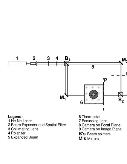
Figure 1: Schematic diagram of the experimental optical setup used for the focal plane and image plane detection techniques. See figure legend for explanation of various parts of the setup.

In the focal plane technique, we exploit the refractive index gradient occurring as the sample’s temperature is raised from below to above the critical temperature $T_{\rm C}$. In the process, a fraction of the heptane diffuses into the nitrobenzene and vice versa. As a result, the refractive index profile, discontinuous below $T_{\rm C}$, takes instead a sigmoidal shape (Fig. 2).

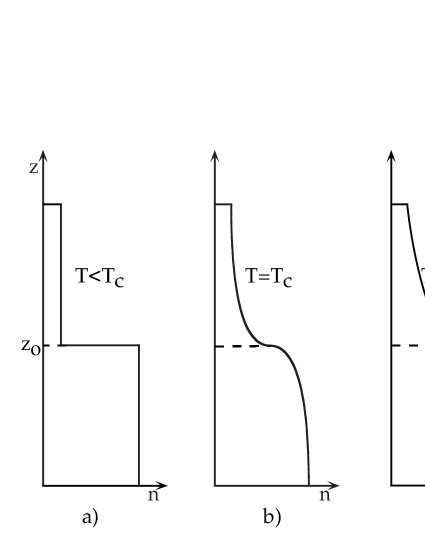
Figure 2: Illustration of the behaviour of the refractive index of a binary mixture as function of cell height at $T<T_{\rm C}$ (a), at $T_{\rm C}$ (b), and $T>>T_{\rm C}$. $z_{0}$ marks the position of the meniscus between the two phases, below $T_{\rm C}$.

The refractive index profile of the sample is probed using a coherent beam of light from a 632.8 nm He-Ne laser, with the beam expanded to approximately 25-mm in diameter and collimated. Light passing through the cell is bent due to the refractive index gradient in the sample. Rays encountering the sigmoidal profile at points with equal absolute value of the curvature are bent through equal angles. If the light is then focussed on a screen by a lens, a diffraction pattern appears in the focal plane of the lens. This diffraction pattern is recorded on photographic film. The number of fringes, $N$, observed in the diffraction pattern at each temperature is directly proportional to the difference in refractive index $\Delta n$ between the two phases: $\Delta n=n_{\rm U}-n_{\rm L}$. It can be shown that, to a good approximation under our experimental conditions [8, 15], $\Delta n$ is proportional to the order parameter of the binary fluid system: $\Delta n=k\Delta\phi$ ($k$ was previously measured as 6.045 [38]; we will discuss this issue further in section 4.4). Therefore, a $\Delta\phi$-versus-temperature graph represents the coexistence curve of the binary mixture and it is suitable for an indirect measurement of the exponent $\beta$.

In the image plane technique, the plane of the recording photographic film is placed on the image plane of the lens also used in the focal plane technique, and the whole refractive index profile of the sample is imaged on the film. As illustrated in Fig. 1, this is achieved by placing the thermostat and sample in one of the beams of a Mach-Zehnder interferometer, while the other beam travels through air. As the refractive index varies considerably with cell height, when the temperature of the sample is in the neighbourhood of the critical temperature, the bottom part of the sample has a larger optical thickness, hence the light of the sample beam that traverses the bottom part of the sample is slowed down more than the light passing through the top part. Therefore, when the waves at P and ${\rm P}^{\prime}$ are recombined and imaged by means of the lens, horizontal interference fringes are observed at the image plane of the lens. The index of refraction as a function of height is mapped in this way. We used this technique to study the sample equilibration time at a set temperature.

2.2 Sample preparation

The liquids were purchased from Fisher Scientific with stated purities of 99% for nitrobenzene and 95% for n-heptane. They were distilled neat (the former under reduced pressure) and brought to an estimated purity of better than 99.9 %, as estimated by gas chromatography as well as by NMR. A mixture was prepared in the proportions of 49.6 wt% n-heptane and 50.4 wt% nitrobenzene, as suggested by earlier studies [16] and the sample was prepared following a method devised and used by this laboratory in the past, with very good results [8].

Several different sample cells were prepared. The cells have a vertically elongated parallelepipedal shape, about 5 cm in height, 1 cm in width, and different depths (the dimension parallel to the He-Ne beam), depending on the light paths wanted for the measurements. In order to observe both the region far from the critical point and the near-critical region with relative ease, the sample cells were chosen to have light paths of 1, 2, 5, and 10 mm (the tolerance of the light paths as quoted by the manufacturer is 0.01 mm; the heights of the fluid in the 1-, 2-, 5-, and 10-mm samples were 34, 35, 37, and 38.5 mm, respectively). In our focal plane measurements, the number of fringes recorded at each temperature decreases as the critical temperature is approached, whereas the error made in counting the fringes is practically constant. Hence, in an effort to reduce the relative error on the fringe count for the data near the critical region, which are usually more significant, samples with longer light paths (5 and 10 mm) are used in that region. On the other hand, as data are taken farther and farther from the critical point, the number of fringes at each datum increases greatly for the same light path ($\simeq 300$ fringes at $T_{\rm C}-T\simeq 0.1$ K with the 10 mm cell), rendering the fringe counting operation more uncomfortable and prone to mistakes in counting. In the temperature region farther from $T_{\rm C}$ the 2- and 1-mm light path sample cells are employed.

2.3 Thermal Control

Thermal control of required stability and uniformity is achieved in two stages combined in a thermostat, whose detailed features are described in reference [17]. The external stage is regulated within $\pm$ 0.1 K, or better, at a temperature, $T_{\rm ext}$, such that $T_{\rm C}-T_{\rm ext}<$ 1 K, by circulating thermostated water in a water jacket system. The second, inner, stage is composed of a copper cylinder, to which heat is applied with heating foils, and of a cell holder, also a copper cylinder fitting snugly within the former. The inner cylinder and the cell holder are in turn placed inside the external stage. After the second heating stage, the temperature can be controlled within about $5\times 10^{-4}$ K. The temperature is measured by a quartz thermometer and by a set of thermistors embedded at various points in the copper cylinder. Both the quartz thermometer and the thermistors were calibrated using a triple point cell to reproduce the triple point of pure water. Tests were performed to ensure that adequate temperature uniformity and stability was achievable with this thermostat. By measurements done under different heating foil configurations, we estimated that thermal gradients along the height of the sample were less than $2\times 10^{-2}$ K/m, which signifies a temperature difference of less than $6\times 10^{-5}$ K along the region of the meniscus, assuming it extends for a few mm in height. In terms of thermal stability, we monitored the temperature of the heater block, as measured by thermistors, for a time span of up to two weeks. In that time, the temperature of the experiment room increased by about 1.3^∘C, while the temperature measured by the thermistors remained stable to within less than $4\times 10^{-4}$ K.

3 Results

3.1 The critical exponent $\beta$

The collected coexistence curve data for the mixture n-heptane+nitrobenzene span 5 decades in terms of the reduced temperature $t$, from $t\simeq 4\times 10^{-7}$ to $t\simeq 4\times 10^{-2}$. Data were taken so as to span the accessible range of temperatures of the mixture, which is around $12.5^{\circ}{\rm C}$ and is bounded by the difference between the critical consolute temperature and the freezing temperature of n-heptane [1]. The data are reported in the online supplemental file accompanying this article.

The coexistence curve data are shown in Fig. 3, where they are expressed as $(\Delta\phi_{H})^{1/0.326}$ vs $t$. In this graph, we have plotted $(\Delta\phi_{H})^{1/0.326}$ as a function of the reduced temperature $t$, instead of the absolute temperature $T$, in order to be able to report on the same graph data from several experimental sequences with slightly different critical temperatures. We discuss below how the different critical temperatures arise.

Figure 3: The coexistence curve data for the binary mixture n-heptane+nitrobenzene expressed as $(\Delta\phi_{H})^{1/0.326}$ as a function of the reduced temperature, where $\Delta\phi_{H}$ is the n-heptane volume fraction. The inset is an enlargement of the critical region.

We anticipated in the introduction that in the vicinity of the critical temperature, the coexistence curve is supposed to be described by the simple scaling law:

$$\Delta\phi=B_{0}t^{\beta}$$ (1)

where $t=1-T/T_{\rm C}$ and $\beta$ is the critical exponent. The “vicinity” of $T_{\rm C}$, or $t=0$—the so-called asymptotic region—has generally been found to be the region with $t<10^{-2}$ for binary liquid mixtures [2]. Translating this to the particular case of n-heptane+nitrobenzene, the region where the simple scaling law should be valid extends to about 3 degrees below $T_{\rm C}$. It should be emphasized, however, that the asymptotic region is not known a priori, nor do we have a theoretical estimate of it. Moreover, in certain circumstances experiments on binary mixtures have suggested that the actual asymptotic region extends only to $t\simeq 10^{-3}$ from the critical temperature [12, 18, 19]. In view of such findings, in the analysis of the present data a narrower asymptotic region $0<t<10^{-3}$ was chosen to find the critical temperature and the order parameter critical exponent $\beta$ from the measured data. Beyond the asymptotic region, correction-to-scaling terms become important:

$$\Delta\phi=B_{0}t^{\beta}\left(1+B_{1}t^{\Delta}+B_{2}t^{2\Delta}+\cdots\right)$$ (2)

where $\Delta$ is the correction-to-scaling critical exponent.

Because it is physically inaccessible, the critical temperature $T_{\rm C}$ must inferred from the measured coexistence curve data. A first estimate of $T_{\rm C}$ is gathered by plotting the raw data as $(\Delta\phi)^{1/\beta}$ versus $T$ in the (expected) asymptotic temperature range, where such a plot is linear. A linear fit to the data intercepts the horizontal axis at $T_{\rm C}$. This value of the critical temperature is then taken as an initial value for a nonlinear least square fit of  (1) to the coexistence curve data in the asymptotic region. In the fit, $\beta$ and $B_{0}$ are used as free parameters. ($T_{\rm C}$ is only allowed to vary within the reasonable range suggested by a careful examination of the coexistence curve near the critical point.) The best values of the parameters found by this nonlinear least square fit are given in Table 1.

Fit	Region	$B_{0}$	$\beta$	$\chi^{2}$
A	$t{\mbox{\lower 2.84526pt\hbox{$\stackrel{{\scriptstyle\textstyle<}}{{\sim}}$}}}10^{-3}$	$1.34\pm 0.01$	(0.326)	$9.8\times 10^{-4}$
B	$t{\mbox{\lower 2.84526pt\hbox{$\stackrel{{\scriptstyle\textstyle<}}{{\sim}}$}}}10^{-3}$	$1.91\pm 0.04$	$0.367\pm 0.002$	$1.3\times 10^{-4}$

Table 1: Parameters values for a nonlinear least square best fit of $\Delta\phi=B_{0}t^{\beta}$ to the volume fraction data of Fig. 3. Quantities in brackets were held fixed during the fit.

As is apparent from the table, the fit obtained with $\beta$ set at the theoretical value of $\beta=0.326$ (fit A) does not seem to represent the data as well as the one where $\beta$ is unconstrained. Instead, the value of the apparent exponent, which produces the best fit is $\beta=0.367\pm 0.006$ (fit B).

Once an estimate of $T_{\rm C}$ has been obtained, a log-log plot of the data in the full temperature range is useful to see if any correction-to-scaling terms would be needed to interpret the data, and whether they should be positive or negative. Also, the slope of the data in the asymptotic region in the log-log plot corresponds to the critical exponent. A log-log plot for the data of Fig. 3 is reported in Fig. 4.

Figure 4: Log-log plot of the order parameter $\Delta\phi_{H}$ versus the reduced temperature $t$. The slope of the data as $t$ tends to zero corresponds to the apparent exponent $\beta$. A line with slope 0.326 is also drawn for comparison.

The slightly decreasing slope at higher values of $t$ indicates that some correction to the simple scaling law are needed and that it will have to have a negative coefficient. This can be seen by performing a nonlinear least square fit of the scaling law (2) to the coexistence curve data of Fig. 3 in the whole range of temperatures studied, by using the best values found in the asymptotic range for the critical temperature $T_{\rm C}$ and for the critical exponent $\beta$ and leaving the coefficient $B_{1}$ free, while the correction-to-scaling exponent $\Delta$ is held fixed at its theoretical value of 0.54 [20, 21]. The line through the data in Fig. 3 corresponds to this fit and the parameters determined by the fit are reported in Table 2, fit C.

Fit	Region	$\beta$	$B_{0}$	$B_{1}$	$\chi^{2}$
C	$t{\mbox{\lower 2.84526pt\hbox{$\stackrel{{\scriptstyle\textstyle<}}{{\sim}}$}}}0.04$	(0.367)	$1.905\pm 0.007$	$-0.96\pm 0.03$	$4.8\times 10^{-4}$
D	$t{\mbox{\lower 2.84526pt\hbox{$\stackrel{{\scriptstyle\textstyle<}}{{\sim}}$}}}0.04$	(0.326)	$1.39\pm 0.01$	$0.11\pm 0.07$	$1.84\times 10^{-3}$
E	$t{\mbox{\lower 2.84526pt\hbox{$\stackrel{{\scriptstyle\textstyle<}}{{\sim}}$}}}0.04$	0.361$\pm$0.002	1.82$\pm$0.03	$-0.81\pm 0.06$	$4.3\times 10^{-4}$

Table 2: Parameters values for a nonlinear least square best fit of $\Delta\phi=B_{0}t^{\beta}\left(1+B_{1}t^{\Delta}+B_{2}t^{2\Delta}\right)$, with $t=(T-T_{\rm C})/T$, to the volume fraction data of Fig. 3. Quantities in brackets were held fixed at the shown value during the fit.

It is evident from the best fit parameters of fits C and D that the scaling law with correction terms works better on the data when $\beta$ is the value found by the simple scaling law used in the asymptotic region (C) than when the theoretical value of $\beta$ is imposed during the fit (D). When the exponent is again treated as a free parameter in the fit, with one correction term (fit E), the value of $\beta$ agrees within error with the one found previously via the simple scaling law.

A different way to perform the analysis of the data and arguably the ultimate verification of the importance of correction terms and of the goodness of the estimate of the measured $\beta$ is achieved by plotting the data in a manner that separates the contribution of the corrections terms from the rest of the terms in the relation (2). If no correction terms are needed to fit the data and the value of the critical exponent is “correct”, a log-log plot of $\Delta\phi_{H}/t^{\beta}$ vs $t$ would distribute the data along a horizontal line (we call this a sensitive plot). Departures from a zero-slope line would then indicate either an “incorrect” value of $\beta$ or the need of correction terms to fit the data, depending on the temperature range. Fig. 5 is a sensitive plot of the coexistence data collected during the experiment with n-heptane+nitrobenzene, where the theoretical value of $\beta=0.326$ was used.

Figure 5: Sensitive log-log plot, $\Delta\phi_{H}$ versus $t$, of the coexistence data on n-heptane+nitrobenzene. The value used for the critical exponent is $\beta=0.326$. A sensitivity scale is also drawn in the graph to indicate the slope the data would preferentially take in the asymptotic region, were they plotted with the value of the exponent corresponding to the indicated slope.

It is evident once again that a value of $\beta$ larger than the theoretical value is necessary to flatten the slope of the data in the asymptotic region. This type of graph can be used to perform a cross check on the values of the critical temperature $T_{\rm C}$ and $\beta$ produced by a nonlinear least square fit to the raw coexistence data of Fig. 3. Starting from some good guesses for $T_{\rm C}$ and $\beta$, one can then vary each of them individually step-by-step until the data of the sensitive plot lies on a horizontal line. The critical temperature will only affect the data very close to $t=0$, while changes in $\beta$ will change the slope of the data on a wider range of $t$. The values of the critical temperature and the critical exponent produced by the experiment will then be the values that make, within experimental error, a zero-slope plot, in the asymptotic region. Moreover, if after this stepwise analysis the data appear distributed along different slopes at different ranges of $t$, this would be an indication that correction terms to the simple scaling law should be included in the fit.

The modern theory of critical phenomena being as widely accepted and successful as it is, it seemed worthwhile to try some fits to the data by using the theoretical value of $\beta$ and adding two correction terms in the scaling law (2). It has been suggested that different exponents for the second correction term can be tried when analyzing coexistence curve data [23, 2, 22]. Further fits to our coexistence data were then tried with the second correction terms being: $B_{2}t^{2\Delta}$, with $\Delta=0.54$, $B^{\prime}_{2}t^{1-\alpha}$, where $\alpha=0.11$ is the specific heat critical exponent, and $B^{\prime\prime}_{2}t^{2\beta}$ with $\beta=0.326$. The rationale behind keeping the choice of the second term open is based on the experimental difficulty to distinguish between a correction exponent that is slightly larger ($2\Delta$) or smaller ($1-\alpha$ or $2\beta$) than one. The results of these fits are reported in Table 3 and they appear to produce worse results than the experimentally measured apparent value of $\beta=0.367\pm 0.006$.

Fit	Region	$\beta$	$B_{0}$	$B_{1}$	$B_{2}$, $B^{\prime}_{2}$, $B^{\prime\prime}_{2}$	$\chi^{2}$
G	$t{\mbox{\lower 2.84526pt\hbox{$\stackrel{{\scriptstyle\textstyle<}}{{\sim}}$}}}0.04$	(0.326)	$1.33\pm 0.03$	$1.5\pm 0.9$	$-7\pm 3$	$1.20\times 10^{-3}$
H	$t{\mbox{\lower 2.84526pt\hbox{$\stackrel{{\scriptstyle\textstyle<}}{{\sim}}$}}}0.04$	(0.326)	$1.32\pm 0.03$	$2\pm 1$	$-6\pm 3$	$1.11\times 10^{-3}$
I	$t{\mbox{\lower 2.84526pt\hbox{$\stackrel{{\scriptstyle\textstyle<}}{{\sim}}$}}}0.04$	(0.326)	$1.30\pm 0.05$	$7\pm 3$	$-9\pm 3$	$9.6\times 10^{-4}$

Table 3: Parameters values for a nonlinear least square best fit of $\Delta\phi=B_{0}t^{\beta}\left(1+B_{1}t^{\Delta}+B_{2}t^{2\Delta}\right)$ (fit G), $\Delta\phi=B_{0}t^{\beta}\left(1+B_{1}t^{\Delta}+B^{\prime}_{2}t^{1-\alpha}\right)$ (fit H), and $\Delta\phi=B_{0}t^{\beta}\left(1+B_{1}t^{\Delta}+B^{\prime\prime}_{2}t^{2\beta}\right)$ (fit I) to the volume fraction data of Fig. 3. Quantities in brackets were held fixed during the fit.

3.2 The critical temperature $T_{\rm C}$

Within each set of order parameter data the temperature was measured using the same thermistor, but different thermistors or other parts of the thermal control electronics were used in different sets. Moreover, as mentioned below in section 2.2, different samples were used to collect the body of data for this experiment.

Systematic experimental studies [24, 25] on the effect of water and acetone impurities in different binary liquid samples (methanol+cyclohexane) show that a percentage volume of water of about 0.1 in the mixture would alter the critical temperature by almost +4 K, while 0.5% of acetone gives a increase of about 2 K. No regular variation of the critical temperature with the different samples was found and the different absolute values measured are all within a fraction of a percent of one another. While it is reasonable to think that both water and acetone impurities are present in the samples (the glass manifolds used to fill the sample cells are cleaned with both distilled water and acetone before making the samples), it is presumed that the amounts of those impurities do not differ much from one sample to the other. For these reasons, the actual critical consolute temperature of n-heptane+nitrobenzene varied somewhat: while for each data set it can be determined to within less than 0.5 mK, its absolute value from our measurements can only be given as $T_{\rm C}=(291.80\pm 0.02)\,{\rm K}$ (18.65 ${}^{\circ}{\rm C}$).

4 Discussion

Due to the marked departure of our measured value of the critical exponent $\beta$ from measurements on other systems as well as from the accepted theoretical value, we have carried out a careful analysis of sources of systematic errors, which may influence this type of measurements. We believe that the influence of other sources of error on the accuracy of our data was minimized by building an ad hoc improved thermostat and by being extremely careful in the conduction of the experiments and in the preparation of the samples.

4.1 The effect of Earth’s gravitational field

Under the influence of Earth’s gravitational field the refractive index vertical profile of a mixture below its consolute critical temperature is in principle distorted from a step-function shape like the one shown in Fig. 2a (references [29, 26, 27, 28] address this issue in binary liquid mixtures in the one-phase region). It is conceivable that the gravity-modified profile would cause the appearance of diffraction fringes even when the system is at a temperature $T<T_{\rm C}$, if the distortion from a pure step-like profile were appreciable. Although, no “unwanted” fringes at temperatures below critical were ever detected in any of the experimental data sets, to study this point in more depth, the image plane method was employed because of its ability to map the index of refraction entire profile (see section 2.1). By counting the fringes as a function of their position on the film (the latter being related to the height in the sample cell), the profile can be plotted. Profile measurements were taken at a temperature above $T_{\rm C}$, after the sample was shaken and therefore in a situation where a homogeneous index of refraction is expected, and below $T_{\rm C}$ roughly 50 hours after the temperature was lowered from above $T_{\rm C}$ (Fig. 6).

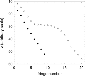
Figure 6: Black diamonds: measurement of the refractive index profile at a temperature $T>T_{\rm C}$ after the sample was shaken to homogenize the phase. White diamonds: analogous measurement taken at a temperature $T<T_{\rm C}$ about 50 hours after the sample was cooled from approximately $8\times 10^{-4}$ K above to approximately $8\times 10^{-4}$ below $T_{\rm C}$.

To ensure that this method is sensitive enough to reproduce a sigmoidal profile if one is present, a measurement was made of the profile after the temperature was raised from below to above $T_{\rm C}$, but without shaking the sample to homogenize the phase. In this situation a profile like Fig. 2b is expected, and is quite clearly measured by this method as is apparent from Fig. 7. From the measured profiles above and below the critical point, there seems to be no evidence of a dramatic deviation of the index of refraction from a homogeneous behaviour, both in the one-phase and the two-phase regions.

Figure 7: Measurement of the refractive index profile at a temperature $T>T_{\rm C}$ after the sample was heated from about 1 mK below to about 1 mK above critical, without shaking it.

Gravitational effect are supposed to be more evident the larger the density difference between the two species of the mixture [29]. The densities of n-heptane and nitrobenzene ($\rho_{\rm H}=0.6837$ and $\rho_{\rm N}=1.2037$, at 20^∘C referred to the density of water at 4^∘C), while not as closely matched as those of other compounds [12], are however less mismatched than at least one other mixture that has revealed no influence of gravitational effect on analogous measurements [18].

4.2 Equilibration

Closely tied to the effect of the terrestrial gravitational field, a very important issue to address is the equilibration time of a binary mixture. As a consequence of the divergences occurring at the critical point, the equilibration time also diverges as the set temperature $T$ tends to $T_{\rm C}$. Hence, the need to wait for an adequately long time after each temperature ($<$$T_{\rm C}$) is set before heating the system through $T_{\rm C}$ to obtain a datum. (And consequently the need for a very stable, as well as accurate thermal control system.) Several other authors have put considerable effort in the study of this phenomenon [26, 27, 28, 29, 30]. From these studies, it appears that the most influential effect on equilibration is the sedimentation flux, which diverges as $(T-T_{C})^{-0.6}$. Only once in the searched literature, however, did we find reference to the effect of this divergence on the two-phase region of a binary mixture, in a study by D. Beysens (within [30]). An order of magnitude calculation along the same lines suggests that in the asymptotic temperature range of our system the relaxation time due to sedimentation can reach several thousand hours (not unlike Beysens’ findings), corroborating serious doubts on the feasibility of carring out meaningful critical phenomena studies of binary liquid mixtures on Earth. Clearly, this effect must have played a role in the experiments reporting results that are more compatible with the renormalization group theory predictions.

We employed the image plane method (section 2.1) to estimate the equilibration time of the system, after a temperature change. This was done by monitoring the interference fringes at the image plane of the focussing lens with time as the film was moved in the camera. For our purposes, equilibrium was reached when the fringes appeared horizontal on the film. In the most significative measurement performed, the temperature was set at a value $T_{\rm i}$ slightly above $T_{\rm C}$ and held there for about two hours, it was then decreased to a temperature $T_{\rm f}$ below $T_{\rm C}$, such that $T_{\rm i}-T_{\rm f}{\mbox{\lower 2.84526pt\hbox{$\stackrel{{\scriptstyle\textstyle<}}{{\sim}}$}}}5\times 10^{-4}$ K. The system was kept at this temperature and the fringes recorded on film for several days. While the chart recorder track of the thermistors output showed that $T_{\rm f}$ was reached about 20 minutes after it was set, the fringes on the film do not appear to flatten to a horizontal slope until about 50 hours later.

The coexistence curve data close to $T_{\rm C}$ were all taken after an equilibration time of about 50 hours, while for the rest of the data the equilibrium time allowance was between 10 and 20 hours.

In principle, data taken before equilibrium is reached would cause one to measure a smaller number of fringes than the “true” number at a given temperature, hence a smaller value of the order parameter $\Delta\phi$. This would, in turn, suggest that waiting a longer time would yield a more curved coexistence curve near $T_{C}$ and hence a “more correct” value for $\beta$.

4.3 Wetting

There is some evidence that in binary mixtures one of the phases wets the walls of the cell containing the sample, as well as the other phase, sometimes surrounding the latter completely [31, 32]. The effect of this phenomenon in the experimental conditions of this work is that the effective thickness of the light path the laser traverses inside the cell is different from the nominal thickness given by the manufacturer. Since the index of refraction, and hence the order parameter, is measured by the number of fringes detected at each temperature divided by the light path length, if the latter is made uncertain by the presence of a wetting film, the consequent refractive index measurements will be affected and rendered unreliable.

By comparing refractive index measurements taken with cells of different thicknesses, the effect of a possible wetting layer can be monitored. Assuming the wetting layer that forms has the same thickness regardless of the nominal light path of the cell, if the data taken with different cells overlap within experimental error, we can neglect the influence of the wetting layer. The coexistence curve measurements were performed with different cell thicknesses to be able to map the whole range of $t$ available for n-heptane+nitrobenzene with equal ease and accuracy. Those measurements as reported in Fig. 4 and Fig. 5 indicate that the data indeed all seem to follow the same pattern. Within the accuracy of the measurements the data overlap, indicating that if a wetting film is present, it is, however, unmeasurable in these experiments.

It is also worth emphasizing that there are indications from other observations [18, 24, 25] and theoretical predictions [33] that wetting behaviour occurs usually at temperatures several degrees below the critical temperature, a region of the coexistence curve with which one is less concerned when determining the critical exponent $\beta$.

4.4 Choice of order parameter

As described above, we use index of refraction measurements to extract the volume fraction information to determine the coexistence curve of our mixture. In doing this three assumptions are made. The first is that the index of refraction does not present any singular behaviour at the critical point. There are theoretical studies [37, 34, 35, 36] and experimental observations dealing with this issue, both showing that any anomaly in the refractive index at the critical point is below 100 ppm, less than the resolution of these experiments. In the case of n-heptane+nitrobenzene, measurements were made in earlier studies to ascertain the goodness of the proportionality relationship between the mixture volume fraction and the order parameter [38]. The proportionality factor was found to be constant within about 0.1% in the temperature range of the two-phase region of n-heptane+nitrobenzene. As such proportionality factor depends on the refractive index of the two phases of the mixture (see, for example, the reference within [15]), we feel safe in the assumption that in our system, too, any refractive index anomalies are likely not influential.

The second assumption made is that of zero mixing volume. In other words, when the two individual species, H and N, are joined together to form the mixture it assumed that their volumes, $V_{{\rm H}}$ and $V_{{\rm N}}$, simply add, while in general it is to be expected that $V_{{\rm mixture}}=V_{{\rm H}}+V_{{\rm N}}\pm|V_{{\rm E}}|$, where $V_{{\rm E}}$ is called the excess volume and it can be positive or negative. Experimental studies on two systems where $V_{{\rm E}}\neq 0$ have shown that this had no consequences on the measured critical exponent $\beta$ [40, 39].

Thirdly, it is assumed that the Lorentz-Lorenz relation remains valid for binary mixtures to the same extent as it valid for pure fluids, for which it holds within about 1%, at least in the neighbourhood of the critical point. According to an experiment aimed at determining the validity of this assumption [40, 41, 42], the Lorentz-Lorenz relation is verified within 0.5%, when the volume loss upon mixing is considered.

We have assumed that the above assumptions are valid for the results obtained with this system, although no measurements were carried out on it to verify such assumptions.

5 Summary and conclusions

Our measurement of the coexistence curve power law critical exponent for the mixture n-heptane+nitrobenzene as the temperature $T\rightarrow T_{c}$ yields an apparent value of $\beta=0.367\pm 0.006$, consistently higher than the accepted theoretical value of $\beta_{\rm theory}\simeq 0.326\pm 0.002$ [7]. In an effort to find a reason for this discrepancy in some experimental flaw, the known potential sources of systematic error were carefully analyzed. In this process, the image plane optical technique was employed to measure the profile of the index of refraction of the binary liquid sample in a way that we had not tried before. The results are interesting in that the shape of the refractive index vertical gradient can be mapped directly by this technique. The relatively new use of this optical tool, as well as employment of an improved thermal control apparatus for the reported measurements have helped rule out that surface wetting by one of the phases, the influence of other effects such as impurities in the samples, and the exact definition of the order parameter could be responsible for the discrepancy between the measured and the theoretically predicted exponent $\beta$. A quick literature survey revealed one other recent report of a similarly high value for $\beta$ from an experiment [43]. However, in that work, there appears no attempt to find a reasonable explanation for the result.

Perhaps, two effects remain as candidate culprits for the high value of $\beta$ we measured. On the one hand is the equilibration time issue. It is somewhat unclear (from this work and previous literature [26, 27, 28, 29, 30]) whether and to what extent the influence of the gravitational field on the equilibration time of this mixture would affect the final outcome of our experiments. Estimates of equilibration times for a given system may vary by an order of magnitude (see, for example, remarks in [27] about observations obtained in [26]). Even in the least consevative case, those estimates would indicate that our equilibrium time allowances were too short and hence that some of our measurements, closer to the critical point, were performed before equilibrium was reached. Should that be indeed the case, while it would leave open a potential explanation for the discrepancy between our measured value of $\beta$ and its widely accepted value, we would still be unable to explain why the fringes observed in the image plane measurements, aimed at establishing when equilibrium was reached, do become horizontal after a time supposedly shorter than the mixture’s equilibration time (section 4.2).

On the other hand, it is conceivable that the asymptotic temperature range of this system be much closer to the critical point than expected for binary mixtures (or even for pure fluids). Our measurements in this case would suggest that the asymptotic region for this binary mixture would have to extend only to $t<10^{-5}$, a considerably narrower interval than the more commonly observed $t<10^{-3}$.

Acknowledgments

We wish to thank Arman Bonakdarpour for his help in the conduction of parts of the experiment. Many thanks also to the department technicians, Doug Wong and Joe O’Connor for their great help in making our glass manifolds, and to Tim Dainard and Bill Goldring for the distillation of the mixture samples. N. F. wishes to thank Professor Ian Affleck for helpful discussions. This work was supported in part by National Sciences and Engineering Research Council (NSERC) of Canada grants to D. A. B.

References

- [1] The Merck Index, Merck & Co., Inc. (1983),pp. 674 and 945.
- [2] A. Kumar, H. R. Krishnamurthy and E. S. R. Gopal, Physics Reports (Review Section of Physics Letters) 98, 58 (1983).
- [3] J. V. Sengers and J. M. H. Levelt-Sengers, Ann. Rev. Phys. Chem. 37, 189 (1986)
- [4] There do exist binary liquid systems in nature which display an inverse behaviour, namely miscibility below the critical temperature and immiscibility above. However, they usually belong to the category of systems with two critical points, lower and upper, where the mixture has its two-phase region between the two critical temperatures.
- [5] To answer the question of which kind of concentration is best suited for the order parameter, the established trend is to use an order parameter the quantity that renders the coexistence curve more symmetric, in order to be able to compare experimental results with the lattice gas model predictions[2]. Experience suggests that the volume fraction usually yields more symmetric coexistence curves. Moreover, the quantity that is usually measured in our binary liquid experiments is the index of refraction difference between the two phases, which turns out to be proportional to the volume concentration.
- [6] F. J. Wegner, Phys. Rev. B 5, 4529 (1972).
- [7] R. Guida and J. Zinn-Justin, J. Phys A 31, 8103 (1998); they find and .
- [8] D. A. Balzarini, Can. J. Phys. 53, 499 (1974).
- [9] A. Stein and G. F. Allen, J. Phys. Chem. Ref. Data 2, 443 (1973).
- [10] J. Shelton and D. A. Balzarini, Can. J. Phys. 59, 934 (1981).
- [11] D. Balzarini and M. Burton, Can. J. Phys. 57, 1516 (1979).
- [12] S. C. Greer, Phys. Rev. A 14, 1770 (1976).
- [13] D. A. Balzarini, Ph. D. Thesis, Columbia University, New York, NY, USA, 1968 (unpublished).
- [14] L. R. Wilcox and D. A. Balzarini, J. Chem. Phys. 48, 753 (1968).
- [15] An expression, without approximation, of the direct proportionality relation between the refractive index and the concentration differences between the liquid phases of a binary mixture is derived in D. T. Jacobs, D. J. Anthony, R. C. Mockler and W. J. O’Sullivan, Chem. Phys. 20, 219 (1977). It is supposed to be valid under the assumption of small anomalies in refractive index and density of the liquids.
- [16] H. Brumberger and R. Pancirov, J. Phys. Chem. 69, 4312 (1965).
- [17] N. Fameli, Ph. D. thesis, The University of British Columbia, Vancouver, B. C., Canada, 2000 (unpublished). Sect. 4.4.
- [18] D. T. Jacobs, D. E. Kuhl, and C. E. Selby, J. Chem. Phys. 105, 588 (1996).
- [19] A. G. Aizpiri, J. A. Correa, R. G. Rubio, and M. Dǐaz Peña, Phys. Rev. B 41, 9003 (1990).
- [20] J.-H. Chen, M. E. Fisher, and B. G. Nickel, Phys. Rev. Lett. 48, 630 (1982).
- [21] S.-Y. Zinn, M. E. Fisher, Physica A 226, 168 (1996).
- [22] R. H. Cohn and S. C. Greer, J. Phys. Chem. 90, 4163 (1986).
- [23] M. E. Fisher, private communication.
- [24] J. L. Tveekrem and D. T. Jacobs, Phys. Rev. A 27, 2773 (1983).
- [25] R. H. Cohn and D. T. Jacobs, J. Chem. Phys. 80, 856 (1984).
- [26] S. C. Greer, T. E. Block, and C. M. Knobler, Phys. Rev. Lett. 34, 250 (1975).
- [27] M. Giglio and A. Vendramini, Phys. Rev. Lett. 35, 168 (1975).
- [28] E. Dickinson, C. M. Knobler, V. N. Schumaker, and R. L. Scott, Phys. Rev. Lett. 34, 180 (1975).
- [29] A. A. Fannin Jr. and C. M. Knobler, Chem. Phys. Lett. 25, 92 (1974).
- [30] G. Maisano, P. Migliardo, and F. Wanderlingh, J. Phys. A: Mathematical and General 9, 2149 (1976); D. Beysens, J. Chem. Phys. 71, 2557 (1979); L. A. Bulavin, A. V. Chalyi, A. V. Oleinikova, J. Molecular Liquids 75, 103 (1998).
- [31] M. R. Moldover and J. W. Cahn, Science 207, 1073 (1980).
- [32] P. de Gennes, Rev. Mod. Phys. 57, 827 (1985).
- [33] J. W. Cahn, J. Chem. Phys. 66, 3667 (1977).
- [34] J. V. Sengers, D. Bedeaux, P. Mazur, and S. C. Greer, Physica A (Amsterdam) 104A, 573 (1980).
- [35] C. Pépin, T. K. Bose, and J. Thoen, Phys. Rev. Lett. 60, 2507 (1988).
- [36] D. Beysens and G. Zalczer, Europhys. Lett. 8, 777 (1989).
- [37] C. L. Hartley, D. T. Jacobs, R. C. Mockler, and J. W. O’Sullivan, Phys. Rev. Lett. 33, 1129 (1974).
- [38] M. Sclavo, Laurea Thesis, University of Padua, Padua, Italy, 1991 (unpublished).
- [39] J. Reeder, T. E. Block, and C. M. Knobler, J. Chem. Thermodyn. 8, 133 (1976).
- [40] W. V. Andrew, T. B. K. Khoo, and D. T. Jacobs, J. Chem. Phys. 85, 3985 (1986).
- [41] C. Houessou, P. Guenoun, R. Gastand, F. Perrot, and D. Beysens, Phys. Rev. A 32, 1818 (1985).
- [42] T. Gastand, D. Beysens, and G. Zalczer, J. Chem, Phys. 93, 3432 (1990).
- [43] D. Venkatesu, J. Chem. Phys. 123, 024902 (2005).