New Cyclic Voltammetry Method for Examining Phase Transitions: Simulated Results

Abstract

We propose a new experimental technique for cyclic voltammetry, based on the first-order reversal curve (FORC) method for analysis of systems undergoing hysteresis. The advantages of this electrochemical FORC (EC-FORC) technique are demonstrated by applying it to dynamical models of electrochemical adsorption. The method can not only differentiate between discontinuous and continuous phase transitions, but can also quite accurately recover equilibrium behavior from dynamic analysis of systems with a continuous phase transition. Experimental data for EC-FORC analysis could easily be obtained by simple reprogramming of a potentiostat designed for conventional cyclic-voltammetry experiments.

Keywords: Cyclic-voltammetry experiments; First-order reversal curve; Hysteresis; Continuous phase transition; Discontinuous phase transition; Lattice-gas model; Kinetic Monte Carlo simulation.

1 Introduction

Recent technological developments in electrochemical deposition have made possible experimental studies of atomic-scale dynamics [1]. It is therefore now both timely and important to develop new methods for computational analysis of experimental adsorption dynamics. In this paper we apply one such analysis technique, the first-order reversal curve (FORC) method, to analyze model electrosorption systems with continuous and discontinuous phase transitions. We propose that this electrochemical FORC (EC-FORC) method can be a useful new experimental tool in surface electrochemistry.

The EC-FORC method was originally conceived [2] in connection with magnetic hysteresis. It has since been applied to a variety of magnetic systems, ranging from magnetic recording media and nanostructures to geomagnetic compounds, undergoing rate-independent (i.e., very slow) magnetization reversal [3]. Recently, there have also been several FORC studies of rate-dependent reversal [4, 5, 6]. Here we introduce and apply the FORC method in an electrochemical context.

The FORC analysis is applied to rate-dependent adsorption in two-dimensional lattice-gas models of electrochemical deposition. We study the dynamics of two specific models, using kinetic Monte Carlo (KMC) simulations. First, we consider a lattice-gas model with attractive nearest-neighbor interactions (a simple model of underpotential deposition, UPD), being driven across its discontinuous phase transition by a time-varying electrochemical potential. Second, we study a lattice-gas model with repulsive lateral interactions and nearest-neighbor exclusion (similar to the model of halide adsorption on Ag(100), described in Refs. [7, 8, 9, 10]), being similarly driven through its continuous phase transition. Some preliminary results of this work have been submitted for publication elsewhere [11].

The rest of this paper is organized as follows. In Sec. 2 the FORC method is explained. The lattice-gas model used both for systems with continuous and discontinuous transitions is introduced in Sec. 3. In Sec. 4 the dynamics of systems with a discontinuous phase transition are studied. The dynamics of systems with a continuous phase transition are studied in Sec. 5. Finally, a comparison between the two kinds of phase transitions is presented together with our conclusions in Sec. 6.

2 The EC-FORC Method

For an electrochemical adsorption system, the FORC method consists of saturating the adsorbate coverage $\theta$ in a strong positive electrochemical potential $\bar{\mu}$ (proportional to the electrode potential, with the same sign for anions and opposite sign for cations) and, in each case starting from saturation, decreasing $\bar{\mu}$ at a constant scan rate $\Omega$ to a series of progressively more negative “reversal potentials” $\bar{\mu}_{r}$. (See Fig. 1).

Figure 1: (a) Schematic diagram of two first-order reversal curves (FORCs) $\theta(\bar{\mu}_{r},\bar{\mu}_{i})$, separated by the reversal-field step size $\Delta\bar{\mu}_{r}$ (solid lines). The dotted lines represent the major hysteresis loop. (b) The corresponding voltammetric currents, $i(\bar{\mu}_{r},\bar{\mu}_{i})\propto\partial\theta/\partial\bar{\mu}_{i}$.

Subsequently, the potential is increased back to the saturating value at the same rate $\Omega$ [3]. The method is thus a simple generalization of the standard cyclic voltammetry (CV) method, in which the negative return potential is decreased for each cycle. This produces a family of FORCs, $\theta(\bar{\mu}_{r},\bar{\mu}_{i})$, where $\theta$ is the adsorbate coverage and $\bar{\mu}_{i}$ is the instantaneous potential during the increase back toward saturation. Alternatively, as it is usually done in CV experiments, one can record the family of voltammetric currents,

$$i(\bar{\mu}_{r},\bar{\mu}_{i})=-\gamma e\frac{{\rm d}\bar{\mu}_{i}}{{\rm d}t}\frac{\partial\theta}{\partial\bar{\mu}_{i}}\;,$$ (1)

where $\gamma$ is the electrosorption valency [12, 13, 14] and $e$ is the elementary charge. Although we shall not discuss this further here, it is of course also possible to fix the negative limiting potential and change the positive return potential from cycle to cycle.

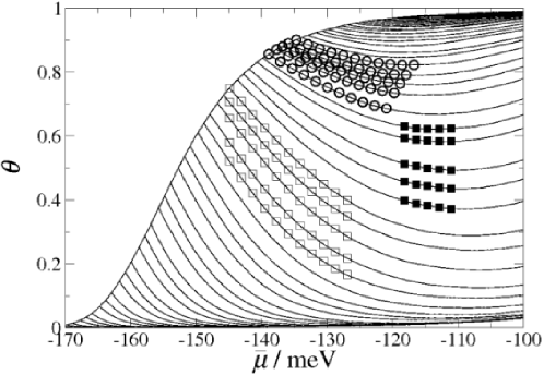
Figure 2: A subset of the family of FORCs. The circled points are an example of the ‘slanted’ $5\times 11$ array of data points used to calculate $\rho$ from $\theta(\bar{\mu}_{r},\bar{\mu}_{i})$. The filled squares represent a ‘square’ $5\times 5$ array and the hollow squares represent a ‘square’ $5\times 11$ array. See discussion in the text.

The family of FORCs consists of $N$ FORCs measured at values of $\bar{\mu}_{r}$ that are evenly spaced by $\Delta\bar{\mu}_{r}$. Each of these FORCs has data points measured at the (in general different) constant spacing $\Delta\bar{\mu}_{i}$ [3]. It is further useful to calculate the FORC distribution,

$$\rho=-\frac{1}{2}\frac{\partial^{2}\theta}{\partial\bar{\mu}_{r}\,\partial\bar{\mu}_{i}}=\frac{1}{2\gamma e({\rm d}\bar{\mu}_{i}/{\rm d}t)}\frac{\partial i(\bar{\mu}_{r},\bar{\mu}_{i})}{\partial\bar{\mu}_{r}}\;,$$ (2)

which measures the sensitivity of the dynamics to the progress of reversal along the outermost hysteresis loop or major loop.

The details of the calculation of $\rho$ depend on whether the measured quantity is the coverage $\theta(\bar{\mu}_{r},\bar{\mu}_{i})$, which is the most convenient in simulation studies, or the voltammetric current $i(\bar{\mu}_{r},\bar{\mu}_{i})$, which would be most usual in CV experiments. In the latter case, the calculation involves simple one-dimensional numerical differentiation with respect to $\bar{\mu}_{r}$, e.g. $\rho=[2\gamma e({\rm d}\bar{\mu}_{i}/{\rm d}t)]^{-1}[i(\bar{\mu}_{r}+\Delta\bar{\mu}_{r},\bar{\mu}_{i})-i(\bar{\mu}_{r},\bar{\mu}_{i})]/\Delta\bar{\mu}_{r}$. Geometrically it is proportional to the vertical distance between the current traces. (See Fig. 1(b).)

In the case that $\theta(\bar{\mu}_{r},\bar{\mu}_{i})$ is the measured quantity, as in the simulations presented here, the calculation of $\rho$ is somewhat more complicated. An array of data points $\theta(\bar{\mu}_{r},\bar{\mu}_{i})$ from consecutive FORCs is used to calculate $\rho$ as shown in Fig. 2. A polynomial surface is fit to this array of data points to provide a functional form of $\theta(\bar{\mu}_{r},\bar{\mu}_{i})$, the mixed partial derivative of which is proportional to $\rho$ as given by Eq. (2). Away from the major hysteresis loop, the array of data points used to calculate $\rho$ can be taken to be ‘square’, i.e., to start and end at the same value of $\bar{\mu}_{i}$ for each of the FORCs involved (squares in Fig. 2). Close to the major loop, this is not geometrically possible. As shown in Fig. 2, we therefore used a ‘slanted’ array of data points to calculate $\rho$. To obtain the values of $\rho$ at grid points other than the center point of the grid ($\bar{\mu}_{i}$, closer to $\bar{\mu}_{r}$) we used a third-order polynomial to fit $\theta(\bar{\mu}_{r},\bar{\mu}_{i})$. This allows the evaluation of the mixed partial derivative $\rho$ at all points of the grid, while a second-order polynomial fit only allows the evaluation of $\rho$ at the center point. For consistency and convenience, a third-order polynomial was used with the three kinds of grids described above and at all points close to and away from the major loop. The three kinds of grids were compared for points away from the major hysteresis loop. While the larger $5\times 11$ grids (‘square’, and ‘slanted’) produced very similar and smooth FORC diagrams, the FORC diagram produced by the $5\times 5$ grid was more noisy. Consequently, in the results shown in this paper, the $5\times 11$ ‘slanted’ grid was used to calculate $\rho$ from $\theta(\bar{\mu}_{r},\bar{\mu}_{i})$ for all values of the arguments.

Another approach to calculating $\rho$ near the major loop would be to use an ‘extended FORC diagram’ [15], for which a square grid of points can be used even near the major loop, but where the delta function normalization term (See Footnote 1) will automatically be included by the polynomial fitting procedure described above. The methods for calculating $\rho$ that are described here, are quite straightforward, but also rather slow. A faster method is based on the Savitzky-Golay smoothing algorithm [16, 17]. It is described in Ref. [18].

The FORC distribution is usually displayed as a contour plot called a ‘FORC diagram.’ A positive value of $\rho$ indicates that the corresponding FORCs are converging with increasing $\bar{\mu}_{i}$, while a negative value indicates divergence. The physical significance of the sign of $\rho$ will become clearer when we apply the EC-FORC method to discontinuous and continuous phase transitions in Secs. 4 and  5, respectively.

3 Model

KMC simulations of lattice-gas models, where a Monte Carlo step (MCS) corresponds to one attempt to cross a free-energy barrier, have been used to simulate the kinetics of electrochemical adsorption in systems with both discontinuous [9, 10, 19, 20] and continuous [7, 21] phase transitions. The energy associated with a lattice-gas configuration is described by the grand-canonical effective Hamiltonian for an $L\times L$ square system of adsorption sites,

$${\mathcal{H}}=-\sum_{i<j}\phi_{ij}c_{i}c_{j}-\bar{\mu}\sum_{i=1}^{L^{2}}c_{i}\;,$$ (3)

where $\sum_{i<j}$ is a sum over all pairs of sites, $\phi_{ij}$ are the lateral interaction energies between particles on the $i$th and $j$th sites measured in meV/pair, and $\bar{\mu}$ is the electrochemical potential measured in meV/atom. The local occupation variables $c_{i}$ can take the values 1 or 0, depending on whether site $i$ is occupied by an ion (1) or solvated (0). The sign convention is chosen such that $\bar{\mu}>0$ favors adsorption. Negative values of $\phi_{ij}$ denote repulsion, while positive values of $\phi_{ij}$ denote attraction between adsorbate particles on the surface. In addition to adsorption/desorption steps, we include diffusion steps that have a free-energy barrier comparable to the adsorption/desorption free-energy barrier [7].

The dynamics of the model are studied by a KMC simulation with the computational time unit of one Monte Carlo Step per Site (1 MCSS = $L^{2}$ MCS). For a discussion of the relation between this simulated time unit and real, physical time, see Ref. [7]. In each MCS of the simulation, an adsorption site is chosen at random and a move (adsorption, desorption, or diffusion) is attempted. The transition rates from the present configuration to the set of new possible configurations are calculated. A weighted list of the probabilities for accepting each of these moves during one MCS is constructed using Eq. (5) below, and used to calculate the probabilities $R\rm{(F|I)}$ of the individual moves between the initial state $\rm I$ and final state $\rm F$. The probability for the system to remain in the initial configuration at the end of the time step is consequently $R\rm{(I|I)}=1-$$\Sigma_{\rm F\neq I}R\rm{(F|I)}$ [7, 8].

Using a thermally activated, stochastic barrier-hopping picture, the energy of the transition state for a microscopic change from an initial state $\rm I$ to a final state $\rm F$ is approximated by the symmetric Butler-Volmer formula [22, 23, 24]

$$U_{\rm T_{\lambda}}=\frac{U_{\rm I}+U_{\rm F}}{2}+\Delta_{\lambda}\;.$$ (4)

Here $U_{\rm I}$ and $U_{\rm F}$ are the energies of the initial and final states as given by Eq. (3), $\rm T_{\lambda}$ is the transition state for process $\lambda$, and $\Delta_{\lambda}$ is a “bare” barrier associated with process $\lambda$. This process can here be either nearest-neighbor diffusion ($\Delta_{\rm nn}$), next-nearest-neighbor diffusion ($\Delta_{\rm nnn}$), or adsorption/desorption ($\Delta_{\rm a/d}$). The probability per unit time for a particle to make a transition from state $\rm I$ to state $\rm F$ is approximated by the one-step Arrhenius rate [22, 23, 24]

$$\mathcal{R}({\rm F}|{\rm I})=\nu\exp\left(-\frac{U_{\rm T_{\lambda}}-U_{\rm I}}{k_{\rm B}T}\right)=\nu\exp\left(-\frac{\Delta_{\lambda}}{k_{\rm B}T}\right)\exp\left(-\frac{U_{\rm F}-U_{\rm I}}{2k_{\rm B}T}\right),$$ (5)

where $k_{\rm B}$ is Boltzmann’s constant and $T$ is the absolute temperature. Here, $\nu$ is the attempt frequency, which sets the overall timescale for the simulation. We set $\nu$ equal to 1 MCSS^-1, so that the transition probabilities in a single time step (MCS) are given by $R({\rm F}|{\rm I})=\mathcal{R}({\rm F}|{\rm I})L^{-2}$ MCSS. The electrochemical potential $\bar{\mu}$ is changed each MCSS, preventing the system from reaching equilibrium at the instantaneous value of $\bar{\mu}$.

Independent of the diffusional degree of freedom, attractive interactions ($\phi_{ij}>0$) produce a discontinuous phase transition between a low-coverage phase at low $\bar{\mu}$, and a high-coverage phase at high $\bar{\mu}$. In contrast, repulsive interactions ($\phi_{ij}<0$) produce a continuous phase transition between a low-coverage disordered phase for low $\bar{\mu}$, and a high-coverage, ordered phase for high $\bar{\mu}$. Examples of systems with a discontinuous phase transition include underpotential deposition [19, 20, 25], while the adsorption of halides on Ag(100) [7, 8, 21, 26, 27] are examples of systems with a continuous phase transition.

4 Discontinuous Phase Transition

A two-dimensional lattice gas with attractive adsorbate-adsorbate lateral interactions that cause a discontinuous phase transition is a simple model of electrochemical underpotential deposition [19, 20, 25, 28]. Using a lattice-gas model with attractive interactions on an $L\times L$ lattice with $L=128$, a family of FORCs were simulated, averaging over ten realizations for each FORC at room temperature. The lateral interaction energy (restricted to nearest-neighbor) was taken to be $\phi_{ij}=\phi_{\rm nn}=55$ meV, where the positive value indicates nearest-neighbor attraction. For this value of $\phi_{\rm nn}$, room temperature corresponds to $T=0.8T_{c}$, where $T_{c}$ is the critical temperature. The barriers for adsorption/desorption and diffusion (nearest-neighbor only) were $\Delta_{\rm a/d}=\Delta_{\rm nn}=150$ meV, corresponding to relatively slow diffusion [20]. Simulation runs with faster diffusion ($\Delta_{\rm nn}=125$ meV) and the same adsorption/desorption barrier were little different from the results shown in Fig. 3. The reversal electrochemical potentials $\bar{\mu}_{r}$ associated with the FORCs were separated by $\Delta\bar{\mu}_{r}=1$ meV increments in the interval $[-200\,{\rm meV},0\,{\rm meV}]$, and the field-sweep rate was constant at $\Omega=|{\Delta}\bar{\mu}_{i}/{{\Delta}t}|=0.03$ meV/MCSS. The FORCs are shown in Fig. 3(a), with a vertical line indicating the position of the coexistence value of the electrochemical potential, $\bar{\mu}_{0}=-110$ meV, and a filled circle showing the position of the minimum of each FORC. The corresponding voltammetric currents are shown in Fig. 3(b).

In a simple Avrami’s-law analysis, the FORC minima all lie at $\bar{\mu}_{i}=\bar{\mu}_{0}$ [6]. However, in the simulations the minima are displaced. For $\theta>0.5$, the minima occur at $\bar{\mu}_{i}<\bar{\mu}_{0}$, precisely at the points where the tendency to phase-order, which drives local regions of the system toward the nearby metastable state ($\theta\approx 1$), is momentarily balanced by the electrochemical potential, which drives the system toward the distant stable state ($\theta\approx 0$). For $\theta<0.5$, the stable and metastable states are $\theta\approx 1$ and $\theta\approx 0$, respectively, and the same balancing effect explains the FORC minima occurring at $\bar{\mu}_{i}>\bar{\mu}_{0}$. The net effect is a ‘back-bending’ of the curve of minima, as seen in Fig. 3(a).

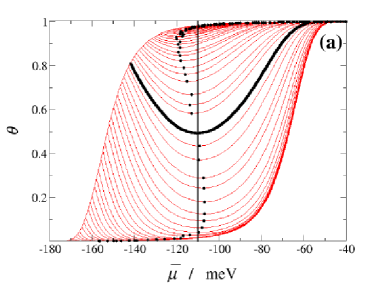
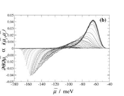
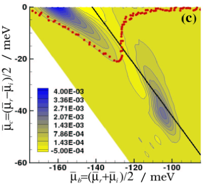
Figure 3: (Color online.) (a) FORCs for a discontinuous phase transition, obtained with scan rate $\Omega=0.03$ meV/MCSS and interactions and barrier heights as given in the text. The vertical line shows the coexistence value of the electrochemical potential, $\bar{\mu}=\bar{\mu}_{0}$. The minimum of each FORC is also shown (filled circles). The thick curve corresponds to the FORC whose minimum lies nearest the coexistence value, $\bar{\mu}_{i}=\bar{\mu}_{0}$. (b) The corresponding voltammetric currents, calculated by numerical differentiation of the FORCs. See Eq. 1. (c) FORC diagram generated from the family of FORCs in (a). The positions of the FORC minima are shown as filled circles. The thick, straight line corresponds to the FORC marked as a thick curve in (a).

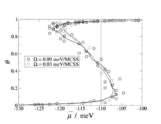
Figure 4: The dependence of the FORC minima on the sweep rate $\Omega$. The figure shows FORC minima for two families of FORCs with different sweep rates ($\Omega=0.03$ and $0.09$ meV/MCSS, respectively). The curves are guides to the eye, obtained by smoothing the data using a first-order Savitzky-Golay filter with a window of 5 points [16, 17].

In Fig 3(c), the FORC diagram is plotted against the variables $\bar{\mu}_{b}=(\bar{\mu}_{r}+\bar{\mu}_{i})/2$ and $\bar{\mu}_{c}=(\bar{\mu}_{r}-\bar{\mu}_{i})/2$. These variables are commonly used in the literature for plotting FORC diagrams [3], as $\bar{\mu}_{b}$ denotes the midpoint between $\bar{\mu}_{r}$ and $\bar{\mu}_{i}$, and $\bar{\mu}_{c}$ is proportional to the distance between these two values of $\bar{\mu}$.

The definition in Eq. (2) implies that the FORC distribution $\rho$ should be negative in the vicinity of the back-bending. This can be readily seen in Fig 3(c). The negative values of $\rho$ reflect a local divergence of the FORCs away from each other as $\bar{\mu}_{i}$ (and time) increases. This can be considered a dynamical instability, caused by the competition between the tendency to phase-order and the effect of the electrochemical potential. When the potential sweep is stopped suddenly at a potential in this unstable region, the subsequent time evolution of $\theta$ is non-monotonic: it first approaches its metastable value, but then reverses and relaxes reliably to its equilibrium value at that potential. The only exception is the point ($\bar{\mu}=\bar{\mu}_{0},\theta=0.5$) along the FORC indicated by bold lines in Fig. 3. It is also interesting to note that the curve connecting the minima of the FORCs resembles the van der Waals loop in the mean-field isotherm of a fluid system below its critical temperature [29], but with an asymmetrical shape about the point ($\bar{\mu}=\bar{\mu}_{0},\theta=0.5$) and with a sweep-rate dependent shape as shown in Fig. 4.

5 Continuous Phase Transition

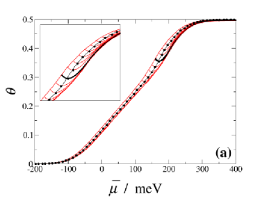
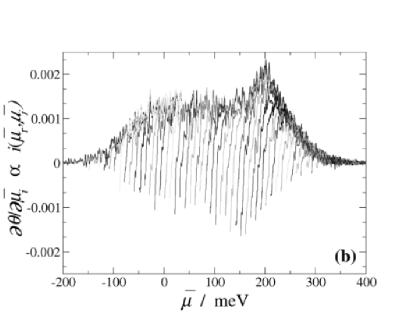
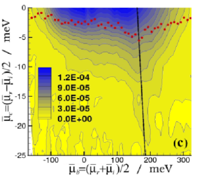
Figure 5: (Color online.) (a) FORCs for a continuous phase transition simulated at a slow scan rate, $\Omega=0.0003$ meV/MCSS. The thin black curve near the middle of the major loop is the equilibrium isotherm. The inset is a magnification of the critical region. The minimum of each FORC is also shown (filled circles). The thick, black curve shows the first FORC which dips below the critical coverage, $\theta_{c}\approx 0.36$. (b) The corresponding voltammetric currents, calculated by numerical differentiation of the FORCs. See Eq. 1. (c) FORC diagram generated from the FORCs in (a). The positions of the FORC minima are shown as filled circles. The thick, straight line corresponds to the FORC marked as a thick curve in (a).

Using the same Hamiltonian, but with long-range repulsive interactions and nearest-neighbor exclusion as appropriate for modeling halide electrosorption on Ag(100) [7, 8, 9, 10], KMC simulations were used to produce the family of FORCs for a continuous phase transition. The reversal potentials $\bar{\mu}_{r}$ were separated by $\Delta\bar{\mu}_{r}=10$ meV increments in the interval $[-200\,{\rm meV},400\,{\rm meV}]$. As in Refs. [7, 9, 10], the repulsive $1/r^{3}$ interactions, with nearest-neighbor exclusion and $\phi_{\rm nnn}=-21$ meV, are calculated with exact contributions for $r_{ij}\leq 3$, and using a mean-field approximation for $r_{ij}>3$. The barriers for adsorption/desorption and nearest- and next-nearest-neighbor diffusion were approximated on the basis of DFT calculations [21] as $\Delta_{\rm a/d}=300$ meV, $\Delta_{\rm nn}=100$ meV, and $\Delta_{\rm nnn}=200$ meV, respectively [7]. Larger values of the diffusion barrier were also used to study the effect of diffusion on the dynamics. A continuous phase transition occurs between a disordered state at low coverage and an ordered state at high coverage [26, 27]. The FORCs, voltammetric currents, and FORC diagram are shown in Fig. 5.

Also indicated in Fig. 5(a) are the FORC minima and the equilibrium isotherm, as calculated in independent equilibrium Monte Carlo simulations. Note that the FORC minima in Fig. 5(a) lie directly on the equilibrium isotherm. This is because such a system has one stable state for any given value of the potential, as defined by the continuous, single-valued equilibrium isotherm. The corresponding voltammetric currents are shown in Fig. 5(b). The uniformly positive value of the FORC diagram in Fig. 5(c) reflects the convergence of the family of FORCs with increasing $\bar{\mu}_{i}$. This convergence results from relaxation toward the equilibrium isotherm, at a rate which increases with the distance from equilibrium. It is interesting to note that, while it is difficult to see at this slow scan rate, the rate of approach to equilibrium decreases greatly along the first FORC that dips below the critical coverage $\theta_{c}\approx 0.36$ (shown in bold in Fig. 5(a)). The FORCs that lie completely in the range $\theta>\theta_{c}$ never enter into the disordered phase, and thus their approach to equilibrium is not hindered by jamming. This is a phenomenon that occurs when further adsorption in a disordered adlayer is hindered by the nearest-neighbor exclusion. As a result, extra diffusion steps are needed to make room for the new adsorbates, and the system follows different dynamics than a system with an ordered adlayer [30]. The FORCs that dip below $\theta_{c}$ enter into the disordered phase, and thus their approach to equilibrium is delayed by jamming. This is reflected in the FORC diagram by the Florida-shaped “peninsula” centered around this FORC in Fig. 5(c).

The effect of jamming is more pronounced at higher scan rates, or with a higher diffusion barrier, where the rate of adsorption is much faster than the rate of diffusion. The family of FORCs and FORC diagram at a higher scan rate, $\Omega=0.01$ meV/MCSS, are shown in Fig. 6, and with a larger diffusion barrier in Fig. 7. In Fig. 6, two distinct groups of FORCs undergoing jammed and unjammed dynamics can be clearly seen. This is reflected in the FORC diagram as a splitting of the “peninsula” into two “islands” of locally maximal values of $\rho$. A similar effect is seen in Fig. 7, since also there the rate of adsorption is much faster than the rate of diffusion (larger diffusion barrier). In addition, Fig. 7(a) shows a slight difference between the FORC minima and the equilibrium curve around the critical coverage. Notice also in Fig. 6(a) that even at a much higher scan rate than in Fig. 5 (nearly two orders of magnitude), the FORC minima still follow the equilibrium curve very accurately. Thus, the EC-FORC method should be useful to obtain the equilibrium adsorption isotherm quite accurately in experimental systems with slow equilibration rates.

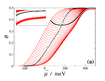
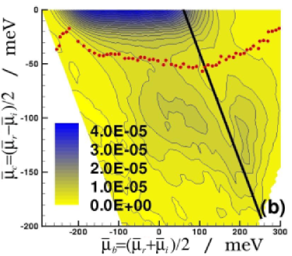
Figure 6: (Color online.) (a) FORCs for a continuous phase transition simulated at a high scan rate, $\Omega=0.01$ meV/MCSS, and the other model parameters as given in the text. The different curves and symbols have the same meanings as in Fig. 5(a). The inset showing the region of large $\bar{\mu}$ and $\theta$ emphasizes the jamming behavior. (b) FORC diagram generated from the FORCs in (a). The different lines and symbols have the same meanings as in Fig. 5(b).

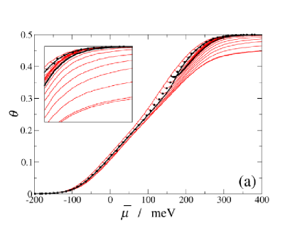
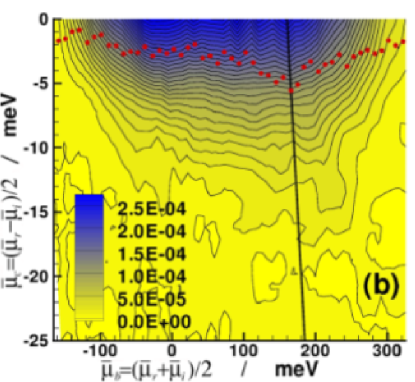
Figure 7: (Color online.) (a) FORCs for a continuous phase transition simulated with $\Omega=0.0003$ meV/MCSS and a large diffusion barrier, $\Delta_{\rm nn}=300$ meV. The other model parameters are as given in the text. The different curves and symbols have the same meanings as in Figs. 5(a) and 6(a). The inset showing the region of large $\bar{\mu}$ and $\theta$ emphasizes the jamming behavior. (b) FORC diagram generated from the FORCs shown in (a). The different lines and symbols have the same meanings as in Figs. 5(b) and 6(b).

6 Comparison and conclusions

Two observations can be made by comparing the FORCs, voltammetric currents, and FORC diagrams for systems with discontinuous and continuous phase transitions. First, the FORC minima in systems with a continuous phase transition correspond closely to the equilibrium behavior, while they do not for systems with a discontinuous phase transition. Thus, FORCs can be used to recover the equilibrium behavior for systems with continuous phase transitions that need a long time to equilibrate. This should be useful in experiments. Second, due to the instability that exists in systems with a discontinuous phase transition, the minima of the family of FORCs in this case form a back-bending “van der Waals loop,” and the corresponding FORC diagram contains negative regions that do not exist for systems with a continuous phase transition. Since experimental implementation of the EC-FORC method should only require simple reprogramming of a potentiostat designed to carry out a standard CV experiment, we believe the method can be of significant use in obtaining additional dynamic as well as equilibrium information from such experiments for systems that exhibit electrochemical adsorption with related phase transitions.

References

- [1] T. Tansel, O.M. Magnussen, Phys. Rev. Lett. 96 (2006) 026101.
- [2] I.D. Mayergoyz, IEEE Trans. Magn. MAG 22 (1986) 603.
- [3] C.R. Pike, A.P. Roberts, K.L. Verosub, J. Appl. Phys. 85 (1999) 6660.
- [4] C. Enachescu, R. Tanasa, A. Stancu, F. Varret, J. Linares, E. Codjovi, Phys. Rev. B 72 (2005) 054413.
- [5] M. Fecioru-Morariu, D. Ricinschi, P. Postolache, C.E. Ciomaga, A. Stancu, J. Optoelectron. Adv. Mater. 6 (2004) 1059.
- [6] D.T. Robb, M.A. Novotny, P.A. Rikvold, J. Appl. Phys. 97 (2005) 10E510.
- [7] I. Abou Hamad, P.A. Rikvold, G. Brown, Surf. Sci. 572 (2004) L355.
- [8] S.J. Mitchell, G. Brown, P.A. Rikvold, Surf. Sci. 471 (2001) 125.
- [9] I. Abou Hamad, Th. Wandlowski, G. Brown, P.A. Rikvold, J. Electroanal. Chem. 554-555 (2003) 211.
- [10] I. Abou Hamad, S.J. Mitchell, Th. Wandlowski, P.A. Rikvold, Electrochim. Acta 50 (2005) 5518.
- [11] I. Abou Hamad, D.T. Robb, P.A. Rikvold, in: D.P. Landau, S.P. Lewis, H.-B. Schüttler (Eds.), Computer Simulation Studies in Condensed-Matter Physics XIX, Springer-Verlag, Berlin, in press.
- [12] K.J. Vetter, J.W. Schultze, Ber. Bunsenges. Phys. Chem. 72 (1972) 920.
- [13] K.J. Vetter, J.W. Schultze, Ber. Bunsenges. Phys. Chem. 72 (1972) 927.
- [14] P.A. Rikvold, Th. Wandlowski, I. Abou Hamad, S.J. Mitchell, G. Brown, Electrochim. Acta (2006), doi:10.1016/j.electacta.2006.07.059
- [15] C.R. Pike, Phys. Rev. B 68 (2003) 104424.
- [16] A. Savitzky, M.J.E. Golay, Anal. Chem. 36 (1964) 1627.
- [17] W.H. Press, A. Teukolsky, W.T. Vetterling, B.P. Flannery, Numerical Recipes in C: The Art of Scientific Computing, Cambridge University Press, Cambridge, 1997, Ch. 14.
- [18] D. Heslop, A.R. Muxworthy, J. Magn. Magn. Mater. 288 (2005) 155.
- [19] S. Frank, D.E. Roberts, P.A. Rikvold, J. Chem. Phys. 122 (2005) 064705.
- [20] S. Frank, P.A. Rikvold, Surf. Sci. 600 (2006) 2470.
- [21] S.J. Mitchell, S. Wang, P.A. Rikvold, Faraday Disc. 121 (2002) 53.
- [22] G. Brown, P.A. Rikvold, S.J. Mitchell, M.A. Novotny, in: A. Wieckowski (Ed.), Interfacial Electrochemistry: Theory, Experiment, and Application, Marcel Dekker, New York, 1999, p. 47.
- [23] H.C. Kang, W.H. Weinberg, J. Chem. Phys. 90 (1989) 2824.
- [24] G.M. Buendía, P.A. Rikvold, K. Park, M.A. Novotny, J. Chem. Phys. 121 (2004) 4193.
- [25] G. Brown, P.A. Rikvold, M.A. Novotny, A. Wieckowski, J. Electrochem. Soc. 146 (1999) 1035.
- [26] B.M. Ocko, J.X. Wang, Th. Wandlowski, Phys. Rev. Lett. 79 (1997) 1511.
- [27] Th. Wandlowski, J. X. Wang, and B. M. Ocko, J. Electroanal. Chem. 500 (2001) 418.
- [28] R.A. Ramos, P.A. Rikvold, M.A. Novotny, Phys. Rev. B 59 (1999) 9053.
- [29] G.W. Castellan, Physical Chemistry, Addison-Wesley, Reading, MA, 1964. Ch. 3.
- [30] J.-S. Wand, P. Nielaba, V. Privman, Mod. Phys. Lett. B 7 (1993) 189.