Quantum phase transition in spin systems studied through entanglement estimators

Abstract

Entanglement represents a pure quantum effect involving two or more particles. Spin systems are good candidates for studying this effect and its relation with other collective phenomena ruled by quantum mechanics. While the presence of entangled states can be easily verified, the quantitative estimate of this property is still under investigation. One of the most useful tool in this framework is the concurrence whose definition, albeit limited to $S=1/2$ systems, can be related to the correlators. We consider quantum spin systems defined along chains and square lattices, and described by Heisenberg-like Hamiltonians: our goal is to clarify the relation between entanglement and quantum phase transitions, as well as that between the concurrence the and the specific quantum state of the system.

1. Introduction

The occurrence of collective behavior in many-body quantum systems is associated with classical and quantum correlations. The latter, whose name is entanglement, cannot be accounted for in terms of classical physics and represents the impossibility of giving a local description of a many-body quantum state. Entanglement is expected to play an essential role at quantum phase transitions (QPT), where quantum effects manifest themselves at all length scales, and the problem has recently attracted an increasing interest [1, 2, 3, 4, 5, 6].

Moreover, entanglement comes into play in quantum computation and communication theory, being the main physical resource needed for their specific tasks [7]. In this respect, the perspective of manipulating entanglement by tunable quantum many-body effects appears intriguing.

In this paper, entanglement estimators are found to give important insight in the physics of $S=1/2$ spin systems, for which the concurrence give quantitative definition of bipartite entanglement. Quantum spin chains and two dimensional lattices in external fields are studied. Two striking features are found: the occurrence of a factorized ground state at a field $\,h_{f}\,$ and that of a QPT at $\,h_{c}>h_{f}\,$, where multipartite entanglement plays an essential role.

The entanglement estimators have been calculated by numerical simulations, carried out in models with linear dimension $\,L\,$, via Stochastic Series Expansion (SSE) Quantum Monte Carlo based on a modified directed-loop algorithm [8]. We have verified that the inverse temperature $\,\beta=2L\,$ is suitable to test the $\,T=0\,$ behaviour.

2. The model

We consider the antiferromagnetic $S=1/2$ XYZ model in a uniform magnetic field:

$${\hat{\cal H}}/J=\sum_{\langle ij\rangle}\Big{[}\hat{S}^{x}_{i}\hat{S}^{x}_{j}+\Delta_{y}\hat{S}^{y}_{i}\hat{S}^{y}_{j}+\Delta_{z}\hat{S}^{z}_{i}\hat{S}^{z}_{j}\Big{]}-\sum_{i}{\bf h}\cdot\hat{\bf S}_{i}~{},$$ (1)

where $J{>}0$ is the exchange coupling, $\langle ij\rangle$ runs over the pairs of nearest neighbors, and ${\bf h}{\equiv}g\mu_{\rm B}{\bf H}/J$ is the reduced magnetic field. The canonical transformation $\hat{S}^{x,y}_{i}{\to}({-}1)^{I}\hat{S}^{x,y}_{i}$ with $I=1(2)$ for $i$ belonging to sublattice $1(2)$, transforms the coupling in the $xy$ plane from antiferromagnetic to ferromagnetic. The Hamiltonian (1) is the most general one for an anisotropic $S=1/2$ system with exchange spin-spin interactions. However, as real compounds usually display axial symmetry, we will henceforth consider either $\Delta_{y}{=}1$ or $\Delta_{z}{=}1$. Moreover, we will apply the field along the $z$-axis, i.e. ${\bf h}{=}(0,0,h)$.

This paper focuses on the less investigated case $\Delta_{z}{=}1$, defining the XYX model in a field. Due to the non-commutativity of the Zeeman and the exchange term, for $\Delta_{y}{\neq}1$ this model is expected to show a field-induced QPT on any D-dimensional bipartite lattice, with the universality class of the D-dimensional Ising model in a transverse field [9]. The two cases $\Delta_{y}{{<}}1$ and $\Delta_{y}{>}1$ correspond to an easy-plane (EP) and easy-axis (EA) behavior, respectively. The ordered phase in the EP(EA) case arises by spontaneous symmetry breaking along the $x$($y$) direction, which corresponds to a finite value of the order parameter $M^{x}$($M^{y}$) below the critical field $h_{\rm c}$. At the transition, long-range correlations are destroyed, and the system is left in a partially polarized state with field-induced magnetization reaching saturation only as $h{\to}\infty$. This picture has been verified so far in D=1 only, both analytically [10]and numerically [2, 11].

Besides its quantum critical behavior, a striking feature of the model Eq. (1) is the occurrence of an exactly factorized ground state for a field $\,h_{\rm f}(\Delta_{y})\,$ lower than the critical field $\,h_{\rm c}$. This feature was previously predicted in Ref. [12] for magnetic chains, and its entanglement behaviour has been studied in Ref. [2]. Our QMC simulations have given evidence [3] for a factorized ground state to occur also in D=2. We have then rigorously generalized the proof of factorization to the most general Hamiltonian Eq. (1) on any 2D bipartite lattice. The proof will be soon reported elsewhere, but we here outline the essential findings in the following. The occurrence of a factorized ground state is particularly surprising if one considers that we are dealing with the $\,S=1/2\,$ case, characterized by the most pronounced effects of quantum fluctuations. However, in the class of models here considered, they are fully uncorrelated[12] at $h=h_{\rm f}$, thus leading to a classical-like ground state.

3. Entanglement estimators

In order to calculate the entanglement of formation [13] in the quantum spin system described by Eq. (1) we make use of the one-tangle and of the concurrence. The one-tangle [14, 15] quantifies the $T=0$ entanglement of a single spin with the rest of the system. It is defined as:

$$\tau_{1}=4\det\rho^{(1)}\,,\>\;\>\rho^{(1)}=(I+\sum_{\alpha}M^{\alpha}\sigma^{\alpha})/2\,;$$ (2)

$\rho^{(1)}\,$ is the one-site reduced density matrix, $M^{\alpha}=\langle\hat{S}^{\alpha}\rangle$, $\sigma^{\alpha}$ are the Pauli matrices, and $\alpha=x,y,z$. In terms of the spin expectation values $M^{\alpha}$, one has:

$$\tau_{1}=1-4\sum_{\alpha}(M^{\alpha})^{2}.$$ (3)

The concurrence [16] quantifies instead the pairwise entanglement between two spins at sites $i$ and $j$, both at zero and finite temperature. For the model of interest, in absence of spontaneous symmetry breaking ($M^{x}=0$) the concurrence reads [15]

$$C_{ij}=2~{}{\rm max}\{0,C_{ij}^{{}^{\prime}},C_{ij}^{{}^{\prime\prime}}\}~{},$$ (4)

where

$$C_{ij}^{{}^{\prime}} = g_{ij}^{zz}-\frac{1}{4}+|g_{ij}^{xx}-g_{ij}^{yy}|~{},$$ (5)

$$C_{ij}^{{}^{\prime\prime}} = |g_{ij}^{xx}+g_{ij}^{yy}|-\sqrt{\left(\frac{1}{4}+g_{ij}^{zz}\right)^{2}-(M^{z})^{2}}~{},$$ (6)

and $g_{ij}^{\alpha\alpha}=\langle\hat{S}_{i}^{\alpha}\hat{S}_{j}^{\alpha}\rangle$ are the static correlators.

One-tangle and concurrence are related by the Coffman-Kundu-Wootters (CKW) conjecture [14], recently proved by Osborne and Verstraete [17], stating that

$$\tau_{1}{\geq}\tau_{2}{\equiv}\sum_{j{\neq}i}C_{ij}^{2}\,,$$ (7)

which expresses the crucial fact that pairwise entanglement does not exhaust the global entanglement of the system, as entanglement can also be stored in $3$-spin correlations, $4$-spin correlations, and so on. Therefore $n$-spin entanglement and $m$-spin entanglement with $m{\neq}n$ are mutually exclusive and this is really a unique feature of entanglement as a form of correlation. The difference with classical correlations is evident.

Due to the CKW conjecture, the entanglement ratio [2] $R{\equiv}\tau_{2}/\tau_{1}{<}1$ quantifies the relative weight of pairwise entanglement, and its deviation from unity shows the relevance of $n$-spin entanglement with $n{>}2$. Although indirect, the entanglement ratio is a powerful tool to estimate multi-spin entanglement.

4. The factorized state

In the one dimensional system described by Eq. (1) the occurence of an exactly factorized ground state for a field $h_{\rm f}(\Delta_{y})$ lower than the critical field $h_{\rm c}$, was predicted in Ref. [12]. In the case of the XYX model, this factorizing field is

$$h_{\rm f}=\sqrt{2(1+\Delta_{y})}\,.$$ (8)

At $h=h_{\rm f}$ the ground state of the model takes a product form $|\Psi\rangle=\bigotimes_{i=1}^{N}|\psi_{i}\rangle$, where the single-spin states $|\psi_{i}\rangle$ are eigenstates of $({\bf n}_{1(2)}\cdot\hat{\bf S})$, where ${\bf n}_{1(2)}$ being the local spin orientation on sublattice 1 (2). Taking ${\bf n}=(\cos\phi\sin\theta,\sin\phi\sin\theta,\cos\theta)$, one obtains [12]

$$\phi_{1}=0\,,\,\phi_{2}=\pi\,,\;\>\theta_{1}=\theta_{2}=\cos^{-1}\sqrt{(1+\Delta_{y})/2}\,.$$ (9)

In particular, for $h=h_{\rm f}$ the spin orientation in the quantum state is exactly the same as in the classical limit of the model made of continuous spins with effective spin length $S_{\rm eff}=1/2$; this means that quantum fluctuations only set the length of the effective classical spin. The factorized state of the anisotropic model continuously connects with the fully polarized state of the isotropic model in a field for $\Delta_{y}=1$ and $h=2$.

In the two-dimensional case, we have found that for any value of the anisotropies $\Delta_{y}$ and $\Delta_{z}$, there exists an ellypsoid in field space

$$\frac{h_{x}^{2}}{(1{+}\Delta_{y})(1{+}\Delta_{z})}{+}\frac{h_{y}^{2}}{(1{+}\Delta_{y})(\Delta_{y}{+}\Delta_{z})}{+}\frac{h_{z}^{2}}{(1{+}\Delta_{z})(\Delta_{y}{+}\Delta_{z})}=4$$ (10)

such that, when $\bf h$ lies on its surface, the ground state of the corresponding model is factorized, $|\Psi\rangle{=}\bigotimes_{i=1}^{N}|\psi_{i}\rangle$. The single-spin states $|\psi_{i}\rangle$ are eigenstates of $({\bf n}_{I}\cdot\hat{\bf S})$, ${\bf n}_{I}$ being the local spin orientation on sublattice $I$. We will hereafter indicate with ${\bf h}_{\rm f}$ (factorizing field) the field satisfying Eq. (10); at ${\bf h}{=}{\bf h}_{\rm f}$, the reduced energy per site is found to be $\epsilon{=}{-}(1{+}\Delta_{y}{+}\Delta_{z})/2$. In the particular case of $\Delta_{z}{=}1$ and ${\bf h}{=}(0,0,h)$, the factorizing field takes the simple expression $h_{\rm f}{=}2\sqrt{2(1{+}\Delta_{y})}$. As for the structure of the ground state, taking ${\bf n}_{I}{=}(\cos\phi_{I}\sin\theta_{I},\sin\phi_{I}\sin\theta_{I},\cos\theta_{I})$, the analytical expressions for $\phi_{I}$ and $\theta_{I}$ are available via the solution of a system of linear equations.

The local spin orientation turns out to be different in the EP and EA cases, being

$$\phi_{1}{=}0\,,\,\phi_{2}{=}\pi\,,\>\>\theta_{1}{=}\theta_{2}{=}\cos^{-1}\sqrt{(1{+}\Delta_{y})/2}\,,$$ (11)

for $\Delta_{y}{<}1$, and

$$\phi_{1}{=}\pi/2\,,\,\phi_{2}{=}{-}\pi/2\,,\>\>\theta_{1}{=}\theta_{2}{=}\cos^{-1}\sqrt{2/(1{+}\Delta_{y})}\,,$$ (12)

for $\Delta_{y}{>}1$.

Despite its exceptional character, the occurrence of a factorized state is not marked by any particular anomaly in the experimentally measurable thermodynamic quantities. On the other hand, entanglement estimators are able to pin down the occurrence of such factorized states with high accuracy, as shown in the following section.

5. Entanglement and quantum phase transitions

The entanglement estimators display a marked anomaly at the factorizing field, where they clearly vanish, as expected. When the field is increased above $h_{\rm f}$, the ground-state entanglement has a very steep recovery, accompanied by the QPT at $h_{\rm c}>h_{\rm f}$. The system realizes therefore an interesting entanglement effect controlled by the magnetic field. This feature is associated with the many-body behavior of the system and it is shown in Fig.1 and Fig.2 for one and two-dimensional systems, respectively.

Fig. 1: One dimensional XYX model with $\Delta_{y}=0.25\,$: $\,\tau_{1}$ and $\tau_{2}$ versus $h$. Insets: entanglement ratio $\tau_{2}/\tau_{1}$ close to the QPT. .

The concurrence terms, are generally short-ranged, and usually do not extend farther than the third neighbor. The longest range of $C_{ij}$ is indeed observed around the factorizing field $h_{\rm f}\,$[18, 19].

The sum of squared concurrences $\tau_{2}$ is seen to be always smaller than or equal to the one-tangle $\tau_{1}$, both for one- and two-dimensional systems. This is in agreement with the CKW conjecture [14]. The total entanglement is only partially stored in two-spin correlations, and it appears also at the level of three-spin entanglement, four-spin entanglement, etc. In particular, we interpret the entanglement ratio

$$R=\tau_{2}/\tau_{1}\,,$$ (13)

as a measure of the fraction of the total entanglement stored in pairwise correlations. This ratio is plotted as a function of the field in the insets of both figures. A striking anomaly occurs at the quantum critical field $h_{c}$, where $R$ displays a very narrow dip. According to our interpretation, this result shows that the weight of pairwise entanglement decreases dramatically at the quantum critical point in favour of multi-spin entanglement. In fact, due to the CKW conjecture, and unlike classical-like correlations, entanglement shows the special property of monogamy, namely full entanglement between two partners implies the absence of entanglement with the rest of the system. Therefore multi-spin entanglement appears as the only possible quantum counterpart to long-range spin-spin correlations occurring at a QPT. This also explains the somewhat puzzling result that the concurrence remains short-ranged at a QPT while the spin-spin correlators become long-ranged [1], and it evidences the serious limitations of concurrence as an estimate of entanglement at a quantum critical point. In turn, we propose the minimum of the entanglement ratio $R$ as a novel estimator of QPT, fully based on entanglement quantifiers.

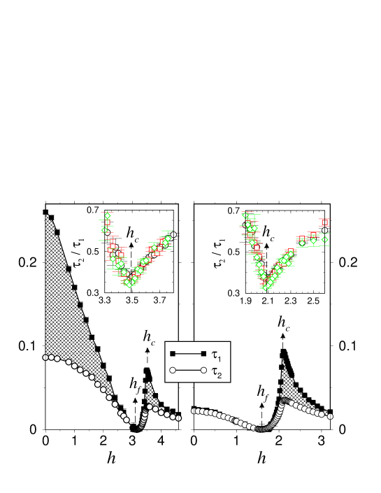
Fig. 2: Two dimensional XYX model: $\tau_{1}$ and $\tau_{2}$ versus $h$. Left panel: easy-plane case ($\Delta_{y}=0.25$); Right panel: easy-axis case ($\Delta_{y}=4$). Insets: entanglement ratio $\tau_{2}/\tau_{1}$ close to the QPT..

6. From spin configurations to entanglement properties

We here analyze the entanglement of formation between two spins, as quantified by the concurrence $C$, in terms of spin configurations. In the simplest case of two isolated spins in the pure state $|\phi\rangle$ the concurrence may be written as $C=|\sum_{i}\alpha_{i}^{2}|$, where $\alpha_{i}$ are the coefficients entering the decomposition of $|\phi\rangle$ upon the magic basis. In this case, it can be easily shown [18] that $C$ extracts the information about the entanglement between two selected spins by combining probabilities and phases relative to some specific two-spin states.

In general, one should notice that a finite probability for two spins to be in a maximally entangled (Bell) state does not guarantee per se the existence of entanglement between them, since this probability may be finite even if the two spins are in a separable state. In a system with decaying correlations, at infinite separation all probabilities associated to Bell states attain the value of $\,1/4\,$, but this of course tells nothing about the entanglement between them, which is clearly vanishing. It is therefore expected that differences between such probabilities, rather than the probabilities themselves give insight in the presence or absence of entanglement.

When the many-body case is tackled, the mixed-state concurrence of the selected spin pair has an involved definition in terms of the reduced two-spin density matrix [16]. We here assume that ${\cal{H}}$ is real, has parity symmetry (meaning that either ${\cal{H}}$ leaves the $z$ component of the total magnetic moment unchanged, or changes it in steps of $2$), and is further characterized by translational and site-inversion invariance.

Let us select two specific spins in the system. We indicate by $p_{\beta}$, with $\beta=1,2,3,4$, the probabilities for the two spins to be in one of the Bell states (maximally entangled), where $\beta=1,2$ (3,4) refers to the parallel (antiparallel) ones. We do also introduce $p_{{{}_{\rm I}}},p_{{{}_{\rm I\!I}}},p_{{{}_{\rm I\!I\!I}}},p_{{{}_{\rm I\!V}}}$, which represent the probabilities for the two spins to be in the (factorized) states of the standard base, where indexes $I$,$I\!I$ ($I\!I\!I$,$I\!V$) refers to the parallel (antiparallel) ones.

It can be shown [18] that $\,C^{\prime}\,$ and $\,C^{\prime\prime}\,$ (as defined in Eqs. (5) and (6) with indexes dropped for simplicity) can be written in terms of the above probabilities:

$$2C^{\prime} = |p_{3}-p_{4}|-2\sqrt{p_{{{}_{\rm I}}}p_{{{}_{\rm I\!I}}}}~{},$$ (14)

$$2C^{\prime\prime} = |p_{1}-p_{2}|-(1-p_{1}-p_{2})=$$ (15)

$$= |p_{1}-p_{2}|-2\sqrt{p_{{{}_{\rm I\!I\!I}}}p_{{{}_{\rm I\!V}}}}~{},$$

where we have used $p_{{{}_{\rm I\!I\!I}}}{=}p_{{{}_{\rm I\!V}}}$ and hence $p_{3}+p_{4}=2p_{{{}_{\rm I\!I\!I}}}=2\sqrt{p_{{{}_{\rm I\!I\!I}}}p_{{{}_{\rm I\!V}}}}$. The expression for $C^{\prime\prime}$ may be written in the particularly simple form

$$2C^{\prime\prime}=2{\rm max}\{p_{1},p_{2}\}-1~{},$$ (16)

telling us that, in order for $C^{\prime\prime}$ to be positive, it must be either $p_{1}>1/2$ or $p_{2}>1/2$. This means that one of the two parallel Bell states needs to saturate at least half of the probability, which implies that it is by far the state where the spin pair is most likely to be found.

Despite the apparently similar structure of Eqs. (14) and (15), understanding $C^{\prime}$ is more involved, due to the fact that $\sqrt{p_{{{}_{\rm I}}}p_{{{}_{\rm I\!I}}}}$ cannot be further simplified unless $p_{{{}_{\rm I}}}=p_{{{}_{\rm I\!I}}}$. The marked difference between $C^{\prime}$ and $C^{\prime\prime}$ reflects the different mechanism through which parallel and antiparallel entanglement is generated when time reversal symmetry is broken; ($p_{{{}_{\rm I}}}\neq p_{{{}_{\rm I\!I}}}$ and hence $M_{z}\neq 0$). In fact, in the zero magnetization case, it is $p_{{{}_{\rm I\!I}}}=p_{{{}_{\rm I}}}=(p_{1}+p_{2})/2$ and hence

$$2C^{\prime}=2{\rm max}\{p_{3},p_{4}\}-1~{},$$ (17)

which is fully analogous to Eq. (16), so that the above analysis can be repeated by simply replacing $p_{1}$ and $p_{2}$ with $p_{3}$ and $p_{4}$.

For $M_{z}\neq 0$, the structure of Eq. (17) is somehow kept by introducing the quantity

$$\Delta^{2}\equiv(\sqrt{p_{{{}_{\rm I}}}}-\sqrt{p_{{{}_{\rm I\!I}}}})^{2}~{},$$ (18)

so that

$$2C^{\prime}=2{\rm max}\{p_{3},p_{4}\}-(1-\Delta^{2})~{},$$ (19)

meaning that the presence of a magnetic field favors bipartite entanglement associated to antiparallel Bell states, $|e_{3}\rangle$ and $|e_{4}\rangle$. In fact, when time reversal symmetry is broken the concurrence can be finite even if $p_{3},~{}p_{4}<1/2$.

¿From Eqs. (16) and (19) one can conclude that, depending on $C$ being finite due to $C^{\prime}$ or $C^{\prime\prime}$, the entanglement of formation originates from finite probabilities for the two selected spins to be parallel or antiparallel, respectively. In this sense we speak about parallel and antiparallel entanglement.

Moreover, from Eqs. (14) and (15) we notice that, in order for parallel (antiparallel) entanglement to be present in the system, the probabilities for the two parallel (antiparallel) Bell states must be not only finite but also different from each other. Thus, the maximally entangled states result mutually exclusive in the formation of entanglement between two spins in the system, which is in fact present only if one of them is more probable than the others. The case $p_{1}=p_{2}=1/2$ ($p_{3}=p_{4}=1/2$) corresponds in turn to an incoherent mixture of the two parallel (antiparallel) Bell states.

The above analysis suggests the first term in $C^{\prime\prime}$ ($C^{\prime}$) to distill, out of all possible parallel (antiparallel) spin configurations, those which are specifically related with entangled parallel (antiparallel) states. These characteristics reinforce the meaning of parallel and antiparallel entanglement.

7. Conclusions

We have analyzed the behaviour of one- and two-dimensional $S=1/2$ antiferromagnets displaying a field-driven quantum phase transition. We have shown that while bipartite entanglement does not show any peculiar feature at the transition, the entanglement ratio $R$ [2], which measure the relevance of bipartite entanglement with respect to the total entanglement content of the system, has a marked dip at criticality: this indicates that multipartite entanglement rules the QPT, $R$ being a powerful tool to detect it.

On the other hand, bipartite entanglement is found to efficiently detect classical-like ground states, even the highly non-trivial ones which are invisible under an analysis based upon standard magnetic observables.

Finally, an interpretation of the analytical expression of the concurrence is given in terms of spin configurations, leading to a deeper insight into the relation between entanglement properties and state configurations in many-body systems.

References

- [1] A. Osterloh et al., Nature (London) 416, 608 (2002).
- [2] T. Roscilde et al., Phys. Rev. Lett. 93, 167203 (2004).
- [3] T. Roscilde et al., Phys. Rev. Lett. 97, 147208 (2005).
- [4] T.J. Osborne et al., Phys. Rev. A 66, 032110 (2002).
- [5] G. Vidal et al., Phys. Rev. Lett. 90, 227902 (2003).
- [6] F. Verstraete et al., Phys. Rev. Lett. 92, 027901 (2004); ibid. 087201 (2004).
- [7] M. A. Nielsen and I. L Chuang, Quantum Computation and Quantum Information, Cambridge Univ. Press, 2000.
- [8] O. F. Syljuåsen et al., Phys. Rev. E 66, 046701 (2002).
- [9] B. K. Chakrabarti et al., Quantum Ising Phases and Transitions in Tranverse Ising Models, Springer, 1996.
- [10] D. V. Dmitriev et al., J. Exp. Th. Phys. 95, 538 (2002).
- [11] J.-S. Caux et al., Phys. Rev. B 68, 134431 (2003).
- [12] J. Kurmann et al., Physica A, 112, 235 (1982).
- [13] C. H. Bennett et al., Phys. Rev. A 54, 3824 (1996).
- [14] V. Coffman et al., Phys. Rev. A 61, 052306 (2000).
- [15] L. Amico et al., Phys. Rev. A 69, 022304 (2004).
- [16] W.K. Wootters, Phys. Rev. Lett. 80, 2245 (1998).
- [17] T.J. Osborne and F. Verstraete, quant-ph/0502176 (2005)
- [18] A. Fubini et al., Eur. Phys. J. D, 38, 563 (2006)
- [19] L. Amico et al., - cond-mat/0602268