Exchange-correlation orbital functionals in current-density-functional theory: Application to a quantum dot in magnetic fields

Abstract

The description of interacting many-electron systems in external magnetic fields is considered in the framework of the optimized effective potential method extended to current-spin-density functional theory. As a case study, a two-dimensional quantum dot in external magnetic fields is investigated. Excellent agreement with quantum Monte Carlo results is obtained when self-interaction corrected correlation energies from the standard local spin-density approximation are added to exact-exchange results. Full self-consistency within the complete current-spin-density-functional framework is found to be of minor importance.

I Introduction

Since its introduction in 1964, density-functional theory (DFT) HK1964 ; KS1965 has become a standard tool to calculate the electronic structure of atoms, molecules, and solids from first principles. Early on, the original DFT formulation has been extended to the case of spin-polarized systems BH1972 which also provides a description of many-electron systems in an external magnetic field. However, in this spin-DFT (SDFT) framework the magnetic field only couples to the spin but not to the orbital degrees of freedom, i.e., the coupling of the electronic momenta to the vector potential associated with the external magnetic field is not taken into account. A proper treatment of this coupling requires extension to current-spin-density-functional theory (CSDFT) VR1987 ; VR1988 in terms of three basic variables: the electron density $n({\bf r})$, the spin magnetization density ${\bf m}({\bf r})$, and the paramagnetic current density ${\bf j}_{p}({\bf r})$. These densities are conjugate variables to the electrostatic potential, the magnetic field, and the vector potential, respectively.

In order to be applicable in practice, DFT of any flavor requires an approximation to the exchange-correlation (xc) energy functional. The use of the local-vorticity approximation, VR1987 ; VR1988 which is an extension of the local spin-density approximation (LSDA), is problematic in CSDFT: the xc energy per particle of a uniform electron gas exhibits derivative discontinuities whenever a Landau level is depopulated in an increasing external magnetic field. This leads to discontinuities in the corresponding xc potential. SV1993 These discontinuities then incorrectly appear when the local values of the inhomogeneous density and vorticity coincide with the corresponding values of the homogeneous electron gas. A popular way to circumvent this problem is to use functionals which interpolate between the limits of weak and high magnetic fields. WR2004b ; SRSHPN2003

Explicitly orbital-dependent functionals, which are successfully used in DFT and collinear SDFT, GKKG2000 ; KK2008 are natural candidates to approximate the xc energy in CSDFT for two reasons: first, they are constructed without recourse to the model of the uniform electron gas and second, they are ideally suited to describe orbital effects such as the filling of Landau levels. In this way, the problem inherent in any uniform-gas-derived functional for CSDFT is avoided in a natural way.

The use of orbital functionals requires the so-called optimized effective potential (OEP) method TS1976 to calculate the effective potentials. The OEP formalism has been recently generalized to non-collinear SDFT SDDHKGSN2006 as well as to CSDFT. PKHG2006 In addition, a larger set of basic densities has been considered in order to include the spin-orbit coupling.B2003 ; RG2006 Recent applications of the OEP method for atoms PKHG2006 and periodic systems SPKSDG07 have indicated that the difference between exact-exchange calculations carried out fully self-consistently within CSDFT or SDFT, respectively, is only minor. These works have also indicated that the inclusion of correlation energies is of particular importance when dealing with current-carrying states.

In this work we consider the OEP formalism within CSDFT in the presence of an external magnetic field. In particular, we focus our attention on two-dimensional semiconductor quantum dots (QDs) RM2002 exposed to uniform and constant external magnetic fields. In addition to the various applications in the field of semiconductor nanotechnology, QDs are also challenging test cases for computational many-electron methods due to the relatively large correlation effects. Moreover, the role of the current induced by the external magnetic field is particularly relevant in QDs elf making them a reference system in CDFT since its early developements. FV1994 Therefore, it is interesting to examine whether the self-consistent solution of CSDFT differs from the result obtained by adding the external vector potential to the SDFT scheme, which amounts to neglecting the xc vector potential of CSDFT.

As expected, we find that the bare exact-exchange (EXX) result is not sufficient to obtain total energies in agreement with numerically accurate quantum Monte Carlo (QMC) results, although a considerable improvement to the Hartree-Fock result is found. However, including the self-interaction corrected LSDA correlation energies to the EXX solution leads to total energies that agree very well with QMC results. In addition, within the given approximations, our results confirm that the role of self-consistent calculations in the framework of CSDFT is only minor. In particular, we observe that accurate total energies and densities can also be obtained by simply modifying the SDFT scheme by including the coupling to the external vector potential. Indeed, this procedure has been employed in the past to partially remedy the lack of good approximate current-dependent functionals. Here, a validation is provided in the more general context of the OEP framework.

This paper is organized as follows. In Sec. II.1 we review the OEP method in CSDFT. The formalism is then adapted to the case of QDs in magnetic fields in Sec. II.2. In Sec. III.1 we discuss details of the numerical procedure before presenting the results of our calculations in Sec. III.2. A brief summary is given in Sec. IV.

II Optimized effective potential method in CSDFT

II.1 General formalism

The Kohn-Sham (KS) equation in CSDFT reads (Hartree atomic units are used throughout unless stated otherwise)

$$\left[\frac{1}{2}\left(\!-i\nabla+\frac{1}{c}{\bf A}_{s}({\bf r})\right)^{2}\!\!\!+v_{s}({\bf r})+\mu_{B}\mbox{\boldmath{$\sigma$}}{\bf B}_{s}({\bf r})\right]\Phi_{k}=\varepsilon_{k}\Phi_{k}.$$ (1)

The three KS potentials are given by

$$v_{s}({\bf r})=v_{0}({\bf r})+v_{H}({\bf r})+v_{xc}({\bf r})+\frac{1}{2c^{2}}\left[{\bf A}_{0}^{2}({\bf r})-{\bf A}_{s}^{2}({\bf r})\right],$$ (2)

$${\bf B}_{s}({\bf r})={\bf B}_{0}({\bf r})+{\bf B}_{xc}({\bf r}),$$ (3)

and

$${\bf A}_{s}({\bf r})={\bf A}_{0}({\bf r})+{\bf A}_{xc}({\bf r}),$$ (4)

where the xc potentials are functional derivatives of the xc energy $E_{xc}$ with respect to the corresponding densities,

$$v_{xc}({\bf r}) = \frac{\delta E_{xc}[n,{\bf m},{\bf j}_{p}]}{\delta n({\bf r})}\;,$$ (5)

$${\bf B}_{xc}({\bf r}) = -\frac{\delta E_{xc}[n,{\bf m},{\bf j}_{p}]}{\delta{\bf m}({\bf r})},$$ (6)

and

$$\frac{1}{c}{\bf A}_{xc}({\bf r}) = \frac{\delta E_{xc}[n,{\bf m},{\bf j}_{p}]}{\delta{\bf j}_{p}({\bf r})}\;,$$ (7)

respectively. The self-consistency cycle is closed by calculating the density

$$n({\bf r})=\sum_{k=1}^{\mathrm{occ}}\Phi_{k}^{\dagger}({\bf r})\Phi_{k}({\bf r})\;,$$ (8)

the magnetization density

$${\bf m}({\bf r})=-\mu_{B}\sum_{k=1}^{\mathrm{occ}}\Phi_{k}^{\dagger}({\bf r})\mbox{\boldmath{$\sigma$}}\Phi_{k}({\bf r})\;,$$ (9)

and the paramagnetic current density

$${\bf j}_{p}({\bf r})=\frac{1}{2i}\!\sum_{k=1}^{\mathrm{occ}}\!\left[\Phi_{k}^{\dagger}({\bf r})\nabla\Phi_{k}({\bf r})\!-\!(\nabla\Phi_{k}^{\dagger}({\bf r}))\Phi_{k}({\bf r})\!\right]\!.$$ (10)

The ground-state total energy of the interacting system can then be computed from

$$E[n,{\bf m},{\bf j}_{p}] = T_{s}[n,{\bf m},{\bf j}_{p}]+U[n]+E_{xc}[n,{\bf m},{\bf j}_{p}]$$ (11)

$$+ \int d{\bf r}\;n({\bf r})v_{0}({\bf r})-\int d{\bf r}\;{\bf m}({\bf r}){\bf B}_{0}({\bf r})$$

$$+ \frac{1}{c}\int d{\bf r}\;{\bf j}_{p}({\bf r}){\bf A}_{0}({\bf r})$$

$$+ \frac{1}{2c^{2}}\int d{\bf r}\;n({\bf r}){\bf A}_{0}^{2}({\bf r}),$$

where $T_{s}$ and $U$ are the kinetic energy of the KS system and the Hartree energy, respectively.

Gauge invariance of the energy functional implies that $E_{xc}$ depends on the current only through the vorticity,

$$\mbox{\boldmath{$\nu$}}({\bf r})=\nabla\times({\bf j}_{p}({\bf r})/n({\bf r})),$$ (12)

i.e., $E_{xc}[n,{\bf j}_{p},{\bf m}]=\bar{E}_{xc}[n,\mbox{\boldmath{$\nu$}},{\bf m}]$. VR1988 This immediately leads to the following relation for the xc vector potential

$$\nabla\left(n({\bf r}){\bf A}_{xc}({\bf r})\right)=0\;.$$ (13)

If one uses an approximate $E_{xc}$ which is given explicitly in terms of the densities, the calculation of the corresponding xc potentials via Eqs. (5)-(7) is straightforward. Here, however, we deal with approximations to the xc energy which are explicit functionals of the KS spinor orbitals $\Phi_{k}$. These functionals are, via the Hohenberg-Kohn theorem, implicit functionals of the densities. In the spirit of the original OEP formalism, the corresponding integral equations for the xc potentials can be derived PKHG2006 by requiring that the effective fields minimize the value of the ground-state total energy (11). Therefore, the functional derivatives of the total energy with respect to the three KS potentials are required to vanish. This procedure leads to three OEP equations which are most conveniently written as PKHG2006

$$\sum_{k=1}^{\mathrm{occ}}\Phi_{k}^{\dagger}({\bf r})\Psi_{k}({\bf r})+h.c.=0,\;$$ (14)

$$-\mu_{B}\sum_{k=1}^{\mathrm{occ}}\Phi_{k}^{\dagger}({\bf r})\mbox{\boldmath{$\sigma$}}\Psi_{k}({\bf r})+h.c.=0\;,$$ (15)

and

$$\frac{1}{2i}\sum_{k=1}^{\mathrm{occ}}\left[\Phi_{k}^{\dagger}({\bf r})\nabla\Psi_{k}({\bf r})-\left(\nabla\Phi_{k}^{\dagger}({\bf r})\right)\Psi_{k}({\bf r})\right]-h.c.=0\;,$$ (16)

where we have defined the so-called “orbital shifts” GKKG2000 ; KP2003a

$$\Psi_{k}({\bf r})=\sum_{\stackrel{{\scriptstyle\scriptstyle j=1}}{{j\neq k}}}^{\infty}\frac{D_{kj}^{\dagger}\Phi_{j}({\bf r})}{\epsilon_{k}-\epsilon_{j}}\;,$$ (17)

with

$$D_{kj}^{\dagger}=\int d{\bf r}^{\prime}\biggl{\{}v_{xc}({\bf r}^{\prime})\Phi_{j}^{\dagger}({\bf r}^{\prime})\Phi_{k}({\bf r}^{\prime})\\ +\frac{1}{2ic}{\bf A}_{xc}({\bf r})\left[\Phi_{j}^{\dagger}({\bf r}^{\prime})\nabla^{\prime}\Phi_{k}({\bf r}^{\prime})-\left(\nabla^{\prime}\Phi_{j}^{\dagger}({\bf r}^{\prime})\right)\Phi_{k}({\bf r}^{\prime})\right]\\ +\mu_{B}{\bf B}_{xc}({\bf r}^{\prime})\Phi_{j}^{\dagger}({\bf r}^{\prime})\mbox{\boldmath{$\sigma$}}\Phi_{k}({\bf r}^{\prime})-\Phi_{j}^{\dagger}({\bf r}^{\prime})\frac{\delta E_{xc}}{\delta\Phi_{k}^{\dagger}({\bf r}^{\prime})}\biggl{\}}.$$ (18)

The orbital shifts $\Psi_{k}$ have the structure of a first-order shift from the unperturbed orbital $\Phi_{k}$ under a perturbation whose matrix elements are given by $D_{kj}^{\dagger}$. Physically, the OEP equations (14)-(16) then imply that the densities do not change under this perturbation. If ${\bf A}_{xc}$ is set to zero, Eqs. (14) and (15) reduce exactly to the OEP equations of non-collinear SDFT. SDDHKGSN2006

Eqs. (14) - (16) form a set of coupled integral equations for the three unknown xc potentials, and they can be solved by a direct computation of the orbital shifts.KP2003a ; SDDHKGSN2006 Alternatively, one can employ the Krieger-Li-Iafrate (KLI) approach as a simplifying approximation SH1953 ; KLI1992b which is known to yield potentials which are very close to the full OEP ones in SDFT. In the following we utilize the KLI approximation in the description of a quasi-two-dimensional semiconductor QD RM2002 in an external magnetic field.

II.2 Application to quantum dots

The QD is described as a many-electron system restricted to the $xy$ plane and confined in that plane by an external parabolic potential $v_{0}=\frac{1}{2}m^{*}\omega_{0}^{2}r^{2}$ with $r^{2}=x^{2}+y^{2}$. Following the most common experimental setup, RM2002 the external magnetic field is defined to be uniform and perpendicular to the $xy$ plane, i.e., ${\bf B}_{0}({\bf r})=\nabla\times{\bf A}_{0}({\bf r})=B_{0}{\bf e}_{z}$ with the gauge ${\bf A}_{0}({\bf r})=B_{0}r{\bf e}_{\theta}/2$. We apply the effective-mass approximation with the material parameters for GaAs, i.e., the effective mass $m^{*}=0.067$, the dielectric constant, $\epsilon^{*}=12.4$, and the effective gyromagnetic ratio $g^{*}=-0.44$.

In QDs the magnetization is parallel to the external field, i.e., these systems show collinear magnetism. Therefore, the KS magnetic field ${\bf B}_{s}$ and the magnetization density have only non-vanishing $z$-components. The Pauli-type KS equation becomes diagonal in spin space and can be decoupled into two separate equations for the spin-up and spin-down orbitals $\varphi_{k\sigma}({\bf r})$. We further assume that the xc potentials preserve the cylindrical symmetry of the problem, i.e.,

$$v_{xc\sigma}({\bf r})=v_{xc\sigma}(r)=v_{xc}(r)\pm\mu_{B}g^{*}B_{xcz}(r),$$ (19)

where the upper signs are for spin-up and lower signs for spin-down electrons, and ${\bf A}_{xc}({\bf r})=A_{xc}(r){\bf e}_{\theta}$. Due to the cylindrical symmetry we can separate the wave function into radial and angular parts as $\varphi_{jl\sigma}({\bf r})=\exp(il\theta)R_{jl\sigma}(r)$, where the radial wave functions $R_{jl\sigma}(r)$ are real-valued eigenfunctions of the Hamiltonian

$$\hat{H}_{sl\sigma}=-\frac{1}{2m^{*}}\left(\frac{\partial^{2}}{\partial r^{2}}+\frac{1}{r}\frac{\partial}{\partial r}-\frac{l^{2}}{r^{2}}\right)+\frac{l}{2}\omega_{c}+m^{*}\frac{\Omega^{2}}{2}r^{2}$$ (20)

$$+\frac{l}{m^{*}c}\frac{A_{xc}(r)}{r}\pm\mu_{B}m^{*}g^{*}B_{0}+v_{H}(r)+v_{xc\sigma}(r)$$

with the total confinement $\Omega=\sqrt{\omega_{0}^{2}+\omega_{c}^{2}/4}$, and the cyclotron frequency $\omega_{c}=B_{0}/m^{*}c$. The radial wave functions are expanded in the basis of eigenfunctions of the corresponding non-interacting problem, i.e., the eigenfunctions of the Hamiltonian (20) with the Hartree and all xc potentials set to zero.

As a consequence of the cylindrical symmetry, the densities are independent of the angle and thus given solely in terms of $r=|{\bf r}|$. Also, only the $\theta$-component of the paramagnetic current density, as the conjugate variable to the vector field in this direction, plays a role, i.e., ${\bf j}_{p}({\bf r})=(j_{p\uparrow}(r)+j_{p\downarrow}(r)){\bf e}_{\theta}$. Instead of using the density and the $z$-component of the magnetization, one employs the spin-up and spin-down densities. Hence, the three densities to be determined are $n_{\uparrow}(r)$, $n_{\downarrow}(r)$, and $j_{p}(r)$.

Consequently, the OEP-KLI equations are given as a $3\times 3$ matrix equation which reads

$${\cal D}(r){\cal V}_{xc}(r)={\cal R}(r),$$ (21)

where the potential vector is given by

$${\cal V}_{xc}(r)=\left(v_{xc\uparrow}(r),v_{xc\downarrow}(r),\frac{1}{c}A_{xc}(r)\right).$$ (22)

The matrix $\cal D$ reads

$${\cal D}=\left(\begin{array}[]{ccc}n_{\uparrow}(r)&0&j_{p\uparrow}(r)\\ 0&n_{\downarrow}(r)&j_{p\downarrow}(r)\\ j_{p\uparrow}(r)&j_{p\downarrow}(r)&N(r)\end{array}\right),$$ (23)

where the densities and current densities are given by

$$n_{\sigma}(r)=\sum_{\{jl\}}^{\mathrm{occ}}R_{jl\sigma}^{2}(r),$$ (24)

$$j_{p\sigma}(r)=\sum_{\{jl\}}^{\mathrm{occ}}\frac{l}{r}R_{jl\sigma}^{2}(r).$$ (25)

The last component $N(r)$ in Eq. (21) reads

$$N(r)=\sum_{\sigma=\uparrow,\downarrow}\sum_{\{jl\}}^{\mathrm{occ}}\frac{l^{2}}{r^{2}}R_{jl\sigma}^{2}(r).$$ (26)

The right-hand-side of Eq. (21) contains functional derivatives of the xc energy. They can be calculated once an approximation to the xc energy is specified. Here, we use the EXX approximation to $E_{xc}$, i.e.,

$$E_{x}^{\mathrm{EXX}}=-\frac{1}{2}\sum_{\sigma=\uparrow,\downarrow}\sum_{\{jl\},\{km\}}^{\mathrm{occ}}$$ (27)

$$\int d^{2}r\,d^{2}r^{\prime}\;\frac{\varphi_{jl\sigma}^{*}({\bf r}^{\prime})\varphi_{jl\sigma}({\bf r})\varphi_{km\sigma}({\bf r}^{\prime})\varphi_{km\sigma}^{*}({\bf r})}{\epsilon^{*}\mid{\bf r}-{\bf r}^{\prime}\mid}\;.$$

The first two components of $\cal R$ on the RHS of Eq. (21) are then given by

$${\cal R}_{1,2}(r) = -\frac{1}{2}\sum_{\{jl\},\{km\}}^{\mathrm{occ}}R_{jl\sigma}(r)R_{km\sigma}(r)$$ (28)

$$\times \int d^{2}r^{\prime}\frac{e^{i\theta^{\prime}(l-m)}R_{jl\sigma}(r^{\prime})R_{km\sigma}(r^{\prime})}{\sqrt{r^{2}+r^{\prime 2}-2rr^{\prime}\cos{\theta^{\prime}}}}$$

$$- \frac{1}{2}\sum_{\{jl\}}^{\mathrm{occ}}n_{jl\sigma}(r)D_{jl,jl,\sigma}^{*}+c.c.,$$

where for ${\cal R}_{1}$ $\sigma=\uparrow$ and for ${\cal R}_{2}$ $\sigma=\downarrow$. The third component is given by

$${\cal R}_{3}(r) = -\frac{1}{2}\sum_{\sigma=\uparrow,\downarrow}\sum_{\{jl\},\{km\}}^{\mathrm{occ}}\frac{l+m}{2}R_{jl\sigma}(r)R_{km\sigma}(r)$$ (29)

$$\times \int d^{2}r^{\prime}\frac{e^{i\theta^{\prime}(l-m)}R_{jl\sigma}(r^{\prime})R_{km\sigma}(r^{\prime})}{\sqrt{r^{2}+r^{\prime 2}-2rr^{\prime}\cos{\theta^{\prime}}}}$$

$$- \frac{1}{2}\sum_{\sigma=\uparrow,\downarrow}\sum_{\{jl\}}^{\mathrm{occ}}j_{pjl\sigma}(r)D_{jl,jl,\sigma}^{*}+c.c.$$

with

$$D_{jl,jl\sigma}^{*} = \int\!d^{2}r\>\left(v_{xc\sigma}(r)+\frac{l}{c}A_{xc}(r)\right)R_{jl\sigma}^{2}(r)$$ (30)

$$+ \sum_{\{km\}}^{\mathrm{occ}}\int\!\!\int d^{2}rd^{2}r^{\prime}e^{i\theta^{\prime}(l-m)}$$

$$\times \frac{R_{jl\sigma}(r^{\prime})R_{km\sigma}(r^{\prime})R_{jl\sigma}(r)R_{km\sigma}(r)}{\sqrt{r^{2}+r^{\prime 2}-2rr^{\prime}\cos{\theta^{\prime}}}}$$

in all three cases.

III Numerical Results

III.1 General remarks

A detailed analysis of Eq. (21) reveals that for a system with a vanishing current the third line of the matrix equation vanishes identically. However, for these states the correct value of the current is already obtained at the level of SDFT as a natural symmetry constraint. In fact, using zero vector potential as the initial value, one can show that it remains zero at each iteration. Hence, one recovers the original SDFT result for non-current carrying states. PKHG2006 On the other hand, for current-carrying states the xc vector potential is always non-vanishing even if one chooses a vanishing vector potential as the initial value.

A closer inspection of the KLI equations shows that they become linearly dependent in the asymptotic region and therefore do not have a unique solution. In our numerical procedure, we take a pragmatic approach to the problem of linearly dependent KLI equations and add a very small positive constant to $N(r)$ in Eq. (26). As the consequence, the limit becomes $A_{xc}(r)\stackrel{{\scriptstyle r\to\infty}}{{\longrightarrow}}0$. In addition, we impose $v_{xc,\sigma}(r)\stackrel{{\scriptstyle r\to\infty}}{{\longrightarrow}}-1/r$. This procedure also limits the possible appearance of numerical artifacts in the KLI potentials resulting from a finite basis-set. Such difficulties have also occurred for open-shell atoms. PKHG2006 ; Diemo Although we face similar problems in QD calculations (see below), we have confirmed that the evaluation of the total energies, densities, and currents is not considerably affected. A further analysis is presented elsewhere. PhD In the context of the full solution of the OEP equations, problems in the computation of the effection potential due to the use of a finite basis-set have been recently analyzed in several works, and different possible solutions have been proposed. TimH ; Staroverov1 ; Staroverov2 ; RohrGri ; Hesselmann

III.2 Examples

Figure 1

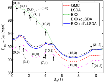
Figure 1: (color online). Total ground-state energy (minus $6\Omega=6\sqrt{\omega_{0}^{2}+\omega_{c}^{2}/4}$) in a six-electron quantum dot as a function of external magnetic field (SI units). The results have been calculated using the exact-exchange (EXX), EXX with LSDA correlation (EXX+cLSDA), and EXX with the corrected LSDA correlation (EXX+c$\uparrow\downarrow$LSDA). The LSDA and quantum Monte Carlo (QMC) results SRSHPN2003 are shown for comparison. The arrows mark the points where the ground-state configuration ($L_{z},S_{z}$) changes.

shows the total energy of a six-electron QD ($\omega_{0}=5$ meV) as a function of $B_{0}$. The kinks correspond to changes in the ground-state configuration ($L_{z},S_{z}$). Apart from the fully-polarized ($S_{z}=3$) states, the EXX energies (dotted line) are considerably too large when compared with the accurate QMC results (dashed line). SRSHPN2003 EXX also leads to an erroneous occurrence of the ($-5,2$) ground-state at $B_{0}=1.5...2.0$ T. However, adding the LSDA correlation AMGB2002 post-hoc to the EXX energies (EXX+cLSDA) yields the correct sequence of states as a function of $B_{0}$. This is a major improvement over the cLSDA-corrected Hartree-Fock calculation which does not give the correct ground states for a similar system. X2000 As expected, the corrections given by cLSDA are largest for the unpolarized state ($0,0$) and smallest for the completely polarized states ($-15,3$) and ($-21;3$). This is due to the fact that the electron exchange has a larger effect on the total energy in systems with a high number of same-spin electrons.

Despite the improvement of EXX+cLSDA over the bare EXX, the result is not satisfactory in comparison with QMC: Figure 1 shows that the energies of EXX+cLSDA are consistently too low by $1.0-1.5$ meV. On the other hand, the agreement between QMC and the conventional LSDA (dash-dotted line) is very good. Hence, taking into account that the EXX is expected to capture the true exchange energy by a good accuracy (the only deviation arising from the missing correlation in the self-consistent solution), our result demonstrates the inherent tendency of the LSDA to cancel out its respective errors in exchange and correlation. This well-known error cancellation is lost when adding LSDA correlation to the EXX result. As expected, the performance of EXX+cLSDA with respect to QMC is at its best in the fully polarized regime ($B_{0}\gtrsim 5$ T), where the exchange contribution in the total energy is relatively at largest.

As a simple cure to the error in EXX+cLSDA, we apply a type of self-interaction correction as first suggested by Stoll and co-workers. stoll The LSDA correlation energy can be improved by

$$E_{\rm c{\uparrow}{\downarrow}LSDA}=E_{\rm cLSDA}$$ (31)

$$- \!\int d^{2}r\,\bigl{\{}n_{\uparrow}({\bf r})\epsilon_{c}[n_{\uparrow},0]+n_{\downarrow}({\bf r})\epsilon_{c}[0,n_{\downarrow}]\bigl{\}}\!,$$

where $\epsilon_{c}[n_{\uparrow},n_{\downarrow}]$ is the correlation energy per electron in the two-dimensional electron gas. AMGB2002 Therefore, in this approximation, denoted as EXX+c${\uparrow}{\downarrow}$LSDA, the correlation energy between like-spin electrons is removed. We emphasize that this contribution is non-zero in the exact treatment and thus cannot be neglected. However, within the LSDA it contains mostly self-interaction energy. Now, we find that EXX+c${\uparrow}{\downarrow}$LSDA (solid line) is very close to QMC, and actually performs better than the conventional LSDA.

Figure 2

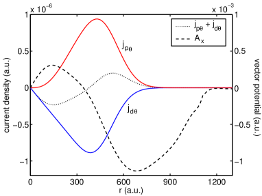
Figure 2: (color online). Angular components of the paramagnetic and diamagnetic currents, $j_{p\theta}$ and $j_{d\theta}$, and their sum for the ($-21,3$) state at $B_{0}=11$ T. The dashed line shows the exchange vector potential for the same configuration.

shows the paramagnetic current $j_{p\theta}$ and the diamagnetic current $j_{d\theta}(r)=n(r)A_{0\theta}(r)/m^{*}$ at $B_{0}=11$ T for the ($-21,3$) state. The total current $j_{\theta}=j_{p\theta}+j_{d\theta}$ changes sign at $r\sim 350$ a.u. due to the existence of a single vortex at the center of the QD. We find the vortex solution in agreement with both LSDA and numerically exact calculations. SHPN2004

In Fig. 2 we also show the exchange vector potential $A_{x}$. The small kink at $r\sim 1100$ a.u. is due to a basis-set problem described in Sec. III.1. The maximum of $|A_{x}|$ is located near the edge of the QD at $r\sim 700$ a.u. However, its relative magnitude with respect to the external vector potential $A_{0}$ is largest at $r\sim 150$ a.u., where we find $|A_{x}/A_{0}|\sim 0.1$. Despite the considerable magnitude of $A_{x}$, we find that its effect on physical quantities like the total energy, density, and current density is practically negligible. In the case presented in Fig. 2, for example, the difference between SDFT and CSDFT total energies is $\sim 0.02\%$. In the context of the OEP method, the minor role of the xc vector potential has been observed for open-shell atoms, PKHG2006 molecules, LHC1995 and extended systems. SPKSDG07 Earlier QD studies in the level of LSDA have also led to similar conclusions. SRSHPN2003

Finally, we point out that, in principle, a given functional should be evaluated with KS orbitals obtained from self-consistent calculations and not in a post-hoc manner as we have done in this work. However, the variational nature of DFT implies that if one evaluates the total energy with a density which slightly differs from the self-consistent density, the resulting change in the energy is of second order in the small deviation of the densities.

IV Summary

We have applied the optimized effective potential method in current-spin-density functional theory to two-dimensional systems exposed to external magnetic fields. We have observed that the bare exact-exchange result (within the KLI approximation) is not sufficient in finding the correct ground-state sequence as a function of the magnetic field, although a considerable improvement over the Hartree-Fock results is found. Adding the correlation energy in the form of the standard local spin-density approximation yields excellent agreement of the ground-state energies with quantum Monte Carlo results, if the spurious self-interaction error is corrected. Moreover, within the specified approximations, we found no considerable differences in total energies and densities when comparing the results obtained using a full-fledged current-spin-density functional theory and a spin-density functional scheme modified to include the coupling to the external vector potential.

- (1) P. Hohenberg and W. Kohn, Phys. Rev. 136, B864 (1964).
- (2) W. Kohn and L. Sham, Phys. Rev. 140, A1133 (1965).
- (3) U. von Barth and L. Hedin, J. Phys. C 5, 1629 (1972).
- (4) G. Vignale and M. Rasolt, Phys. Rev. Lett. 59, 2360 (1987).
- (5) G. Vignale and M. Rasolt, Phys. Rev. B 37, 10685 (1988).
- (6) P. Skudlarski and G. Vignale, Phys. Rev. B 48, 8547 (1993).
- (7) A. Wensauer and U. Rössler, Phys. Rev. B 69, 155302 (2004).
- (8) H. Saarikoski, E. Räsänen, S. Siljamäki, A. Harju, M. J. Puska, and R. M. Nieminen, Phys. Rev. B 67, 205327 (2003).
- (9) T. Grabo, T. Kreibich, S. Kurth, and E. K. U. Gross, in Strong Coulomb Correlations in Electronic Structure: Beyond the Local Density Approximation, edited by V. Anisimov (Gordon & Breach, Tokyo, 2000), pp. 203–311.
- (10) S. Kümmel and L. Kronik, Rev. Mod. Phys. 80, 3 (2008).
- (11) J. D. Talman and W. F. Shadwick, Phys. Rev. A 14, 36 (1976).
- (12) S. Sharma, J. K. Dewhurst, C. Ambrosch-Draxl, S. Kurth, N. Helbig, S. Pittalis, S. Shallcross, L. Nordström, and E. K. U. Gross, Phys. Rev. Lett. 98, 196405 (2007).
- (13) S. Pittalis, S. Kurth, N. Helbig, and E. K. U. Gross, Phys. Rev. A 74, 062511 (2006).
- (14) K. Bencheikh, J. Phys. A: Math. Gen. 36, 11929 (2003).
- (15) S. Rohra and A. Görling, Phys. Rev. Lett. 97, 013005 (2006).
- (16) S. Sharma, S. Pittalis, S. Kurth, S. Shallcross, J. K. Dewhurst, and E. K. U. Gross, Phys. Rev. B 76, 100401(R) (2007).
- (17) S. M. Reimann and M. Manninen, Rev. Mod. Phys. 74, 1283 (2002); L. P. Kouwenhoven, D. G. Austing, and S. Tarucha, Rep. Prog. Phys. 64, 701 (2001).
- (18) E. Räsänen, A. Castro, and E. K. U. Gross, Phys. Rev. B, in print, cond-mat/0801.2373
- (19) M. Ferconi and G. Vignale, Phys. Rev. B 50, 14722 (1994)
- (20) S. Kümmel and J. P. Perdew, Phys. Rev. Lett. 90, 043004 (2003); Phys. Rev. B 68, 035103 (2003).
- (21) R. T. Sharp and G. K. Horton, Phys. Rev. 90, 317 (1953).
- (22) J. B. Krieger, Y. Li, and G.J. Iafrate, Phys. Rev. A 46, 5453 (1992).
- (23) D. Ködderitzsch (private communication).
- (24) S. Pittalis, PhD Thesis, in preparation, Freie Universität Berlin (2008).
- (25) T. H. Burgess, F. A. Bulat, W. Yang, Phys. Rev. Lett. 98, 256401 (2007).
- (26) V. N. Staroverov and G. E. Scuseria, J. Chem. Phys. 124, 141103 (2006).
- (27) V. N. Staroverov and G. E. Scuseria, J. Chem. Phys. 125, 081104 (2006).
- (28) D. R. Rohr, O. V. Gritsenko, and E. J. Baerends, J. Mol. Structure: THEOCHEM 72, 762 (2006).
- (29) A. Hesselmann, A. W. Götz, F. Della Sala, and A. Görling, J. Chem. Phys. 127, 054102 (2007).
- (30) C. Attaccalite, S. Moroni, P. Gori-Giorgi, and G. Bachelet, Phys. Rev. Lett. 88, 256601 (2002).
- (31) W. Xin-Qiang, J. Phys.: Condens. Matter 12, 4207 (2000).
- (32) H. Stoll, E. Golka, and H. Preuss, Theor. Chim. Acta 55, 29 (1980).
- (33) H. Saarikoski, A. Harju, M. J. Puska, and R. M. Nieminen, Phys. Rev. Lett. 93, 116802 (2004).
- (34) A. M. Lee, N. C. Handy, and S. M. Colwell, J. Chem. Phys. 103, 10095 (1995)