Universal and nonuniversal features in the crossover from linear to nonlinear interface growth

Abstract

We study a restricted solid-on-solid (RSOS) model involving deposition and evaporation with probabilities $p$ and $1-p$, respectively, in one-dimensional substrates. It presents a crossover from Edwards-Wilkinson (EW) to Kardar-Parisi-Zhang (KPZ) scaling for $p\approx 0.5$. The associated KPZ equation is analytically derived, exhibiting a coefficient $\lambda$ of the nonlinear term proportional to $q\equiv p-1/2$, which is confirmed numerically by calculation of tilt-dependent growth velocities for several values of $p$. This linear $\lambda-q$ relation contrasts to the apparently universal parabolic law obtained in competitive models mixing EW and KPZ components. The regions where the interface roughness shows pure EW and KPZ scaling are identified for $0.55\leq p\leq 0.8$, which provides numerical estimates of the crossover times $t_{c}$. They scale as $t_{c}\sim\lambda^{-\phi}$ with $\phi=4.1\pm 0.1$, which is in excellent agreement with the theoretically predicted universal value $\phi=4$ and improves previous numerical estimates, which suggested $\phi\approx 3$.

I Introduction

The competition between different growth mechanisms is a characteristic of many real processes and has been the subject of intensive investigation in the last years. Many authors considered competitive growth models in which different dynamic rules are randomly chosen for the aggregation of the incident particles albano1 ; albano2 ; shapir ; julien ; tales ; chamereis ; muraca ; lam ; rdcor ; kolakowska ; bulavin and applications to real systems were suggested shapir ; julien ; yu . Such simplified models may mimic, for instance, the effects of large energy distributions of the incident atoms, which lead to different dynamic behavior as they arrive at the film surface. They usually show crossover effects from one dynamics at small times $t$ or short length scales $L$ to another dynamics at long $t$ or large $L$.

In many cases, a crossover from the Edwards-Wilkinson (EW) ew dynamics to Kardar-Parisi-Zhang (KPZ) growth kpz is observed. The Langevin-type equation

$${{\partial h}\over{\partial t}}=\nu{\nabla}^{2}h+{\lambda\over 2}{\left(\nabla h\right)}^{2}+\eta(\vec{x},t),$$ (1)

known as KPZ equation, is a hydrodynamic description of kinetic surface roughening, where $h$ is the height at the position $\vec{x}$ in a $d$-dimensional substrate at time $t$, $\nu$ represents a surface tension, $\lambda$ represents the excess velocity and $\eta$ is a Gaussian noise kpz ; barabasi with zero mean and variance $\langle\eta\left(\vec{x},t\right)\eta\left(\vec{x^{\prime}},t^{\prime}\right)\rangle=D\delta^{d}\left(\vec{x}-\vec{x^{\prime}}\right)\delta\left(t-t^{\prime}\right)$. When $\lambda=0$ in Eq. (1), we obtain the (linear) EW equation. Thus, if $\lambda$ is very small, the features of EW growth are expected at small times, and a crossover to KPZ behavior is observed at a characteristic time $t_{c}$, when the macroscopic properties are affected by the overall nonlinear character of the process. In this paper, we will analyze universal and nonuniversal features of this crossover in lattice models through analytical and numerical methods.

The roughness (or interface width) $W(L,t)$ is the simplest quantity that indicates crossover effects. In lattice models, it is defined as

$$W(L,t)=\left<{\left[{{1\over{L^{d}}}\sum_{i}{{\left(h_{i}-\overline{h}\right)}^{2}}}\right]}^{1/2}\right>$$ (2)

for deposition in a $d$-dimensional substrate of length $L$ ($h_{i}$ is the height of column $i$ at time $t$, the bar in $\overline{h}$ denotes a spatial average and the angular brackets denote a configurational average). In a typical EW or KPZ system, it scales for small times as

$$W\sim t^{\beta}.$$ (3)

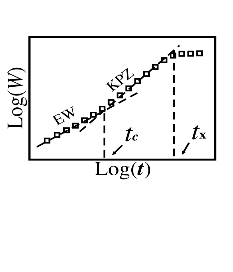
Figure 1: Typical time evolution of the roughness of a system with an EW-KPZ crossover at time $t_{c}$ and saturation time $t_{\times}$.

However, when the crossover EW-KPZ is present, the roughness exhibits two growth regions, characteristic of EW and KPZ scaling ($\beta_{EW}<\beta_{KPZ}$ in any dimension), as shown qualitatively in Fig. 1. At long times, the roughness saturates as

$$W_{sat}\sim L^{\alpha}.$$ (4)

$t_{\times}$ is the crossover time to the steady state or saturation regime, also shown in Fig. 1.

From plausible scaling arguments (reviewed in Sec. III), several authors suggested that, in $d=1$, the EW-KPZ crossover takes place for small $\lambda$ at

$$t_{c}\sim\lambda^{-\phi},$$ (5)

with a universal crossover exponent $\phi=4$ AF ; GGG ; NT ; forrest . However, to our knowledge the best known numerical estimate of this crossover exponent is $\phi\approx 3$. It was obtained by Guo, Grossman and Grant GGG and by Forrest and Toral forrest through numerical solutions of the KPZ equation and data collapse methods. Recent works on lattice models confirmed the expected scaling relations for the growth and saturation regimes of KPZ, even in the presence of the EW-KPZ crossover chamereis , but they were not able to improve the results for the EW regime ($t\ll t_{c}$) or the crossover regions ($t\sim t_{c}$). Thus, neither a numerical confirmation nor a thoroughly justified refutation of the universality of the exponent $\phi=4$ was presented yet.

On the other hand, an universal relation between the coefficient $\lambda$ and parameters of competitive lattice models with the EW-KPZ crossover was recently proposed by Braunstein and co-workers muraca ; lam . They considered processes where the aggregation of incident particles followed the rules of a KPZ lattice model with probability $p$ and the rules of an EW model with probability $1-p$. The most studied representative chamereis ; julien is the competitive model involving ballistic deposition (BD - KPZ class) vold and the Family model, also known as random deposition with surface relaxation (RDSR - EW class) family . The derivation of the corresponding KPZ equation from the stochastic rules of this class of models gives $\lambda\sim p^{2}$ for small $p$ and is confirmed numerically for the RDSR-BD model chamereis .

In the present paper, we will study analytically and numerically a lattice model with the crossover EW-KPZ in $d=1$, which is helpful to clarify the universal and nonuniversal relations in this crossover. The model is a restricted solid-on-solid (RSOS) one kk , in which deposition and evaporation of particles compete with probatilities $p$ and $1-p$, respectively. EW behavior is found for $p=1/2$, and KPZ behavior for $p\neq 1/2$. We will derive analitically the KPZ equation for this process, which exhibits $\lambda\sim q\equiv p-1/2$, where $q$ represents a small relative probability of KPZ growth in the crossover region ($p\approx 1/2$, $q\approx 0$). This linear relation between $q$ and $\lambda$ is confirmed numerically, and contrasts to the parabolic law found in other competitive models. Consequently, the $\lambda-p$ relation in the EW-KPZ crossover is clearly a model-dependent feature and not an universal law. On the other hand, our numerical work will also provide an estimate of the crossover exponent $\phi$ which agrees with the theoretically predicted universal value $\phi=4$, improving previous estimates which failed to confirm that prediction. This exponent is obtained from the scaling of $t_{c}(q)$, which is estimated from the intersection of the EW and KPZ behaviors, as illustrated in Fig. 1. The inherent difficulties of the numerical work, combined with the relatively simple, linear $\lambda-p$ relation, explain why estimating the crossover exponent is usually so hard.

The rest of this work is organized as follows. In Sec. II, we will define precisely the discrete model, analitically derive its associated KPZ equation and confirm numerically the $\lambda\sim q$ relation. In Sec. III we will review the scaling arguments predicting $\phi=4$ and show the details of the numerical analysis which gives $\phi=4.1\pm 0.1$. In Sec. IV we summarize our results and present our conclusions.

II The discrete model and the associated KPZ equation

In our competitive model, the deposit obeys the RSOS condition at any time, i.e. the maximum height difference between neighboring columns is equal to the particle size $a$ kk . In the simulations, we consider $a=1$. At each step of the process, a column of the deposit is randomly chosen. Subsequently, deposition and evaporation attempts are chosen with probabilities $p$ and $1-p$, respectively. When evaporation is chosen, the top particle of that column is removed if the RSOS condition is satisfied after evaporation, otherwise this attempt is rejected. When deposition is chosen, a new particle is deposited at the top of that column if the RSOS condition is satisfied, otherwise this attempt is rejected. The time unit $\tau$ corresponds to $L$ attempts of evaporation or deposition in a substrate with $L$ columns. In the simulations, we considered $\tau=1$.

This model was previously studied numerically by Amar and Family AF2 , in order to show the universality of scaling functions and amplitude ratios for KPZ processes in $d=1$. However, that analysis was restricted to $p\geq 0.75$, consequently far from the region of EW-KPZ crossover.

Now we construct the associated KPZ equation of this process starting from the master equation and performing a Kramers-Moyal expansion vankampen , following the standard method used in Refs. vvedensky ; vvedensky1 ; muraca .

First consider the deposition process according to the RSOS condition. The transition rate $W(H,H^{\prime})$ from the height configuration $H\equiv\{h_{i}\}$ to the configuration $H^{\prime}\equiv\{h_{i}^{\prime}\}$ for this process is

$$W(H,H^{\prime})={1\over\tau}\sum_{k}{w_{k}^{(0)}\delta\left(h_{k}^{\prime},h_{k}+a\right)\prod_{j\neq k}{\delta\left(h_{j}^{\prime},h_{j}\right)}},$$ (6)

where the $\delta$ functions represent the condition that only the height of the column of incidence can be increased and $w_{k}^{(0)}$ describes the condition for aggregation:

$$w_{k}^{(0)}=\Theta\left(h_{k+1}-h_{k}\right)\Theta\left(h_{k-1}-h_{k}\right),$$ (7)

where the $\Theta(x)$ is the unit step function, defined as $\Theta(x)=1$ for $x\geq 0$ and $\Theta(x)=0$ for $x<0$. Consequently, the first and the second transition moments are

$$K_{i}^{(1)}=\sum_{H^{\prime}}{\left(h_{i}^{\prime}-h_{i}\right)W\left(H,H^{\prime}\right)}={a\over\tau}\Theta\left(h_{i+1}-h_{i}\right)\Theta\left(h_{i-1}-h_{i}\right)$$ (8)

and

$$K_{ij}^{(2)}=\sum_{H^{\prime}}{\left(h_{i}^{\prime}-h_{i}\right)\left(h_{j}^{\prime}-h_{j}\right)W\left(H,H^{\prime}\right)}={a^{2}\over\tau}\Theta\left(h_{i+1}-h_{i}\right)\Theta\left(h_{i-1}-h_{i}\right)\delta{\left(i,j\right)}.$$ (9)

For RSOS evaporation, the transition rate and the transition moments are those of Eqs. (7), (8) and (9) with opposite signs in the arguments of the $\Theta$ functions.

The Kramers-Moyal expansion of the master equation for the process provides the stochastic equation vankampen

$${\partial{h_{i}}\over\partial{t}}=K_{i}^{(1)}+\sum_{j}{\sqrt{K_{ij}^{(2)}}\eta_{j}},$$ (10)

where $\eta_{j}$ is a Gaussian white noise with zero mean and co-variance $\langle\eta_{i}(t)\eta_{j}(t^{\prime})\rangle=\delta{\left(i,j\right)}\delta(t-t^{\prime})$. For the competitive model, we obtain

$${\partial{h_{i}}\over\partial{t}}=p{a\over\tau}\Theta\left(h_{i+1}-h_{i}\right)\Theta\left(h_{i-1}-h_{i}\right)-(1-p){a\over\tau}\Theta\left(h_{i}-h_{i+1}\right)\Theta\left(h_{i}-h_{i-1}\right)+D_{i}\eta_{i},$$ (11)

where $D_{i}$ is constant.

In order to pass from the discrete description of the model to its continuum limit, we can use some analytical representation of the step function, which works in some limits. Many regularization for the theta step function have already been suggested, such as the hyperbolic tangent function park , and maximum function vvedensky . This representation is expanded in Taylor series, so that

$$\theta(x)=c_{0}+c_{1}\;x+c_{2}\;x^{2}+\dots$$ (12)

Inserting this expansion in equation (11), we get

$$\frac{dh_{i}}{dt} = p\frac{a}{\tau}\left[c_{0}+c_{1}(h_{i+1}-h_{i})+c_{2}(h_{i+1}-h_{i})^{2}\right]\left[c_{0}+c_{1}(h_{i-1}-h_{i})+c_{2}(h_{i-1}-h_{i})^{2}\right]$$ (13)

$$- (1-p)\frac{a}{\tau}\left[c_{0}+c_{1}(h_{i}-h_{i+1})+c_{2}(h_{i}-h_{i+1})^{2}\right]\left[c_{0}+c_{1}(h_{i}-h_{i-1})+c_{2}(h_{i}-h_{i-1})^{2}\right]$$

$$+ D_{i}\eta_{i}$$

In the continuum limit, $a\to 0$. In this limit, $ac_{1}$ tends to a finite, nonzero value, since the angular coeficient $c_{1}$ in the expansion of the theta function (Eq. 12) is of order $1/a$. Moreover, $a/\tau\to const$, since this is the random growth velocity. We replace $h_{i}(t)$ by a smooth function $h(x,t)$, whose coarse-grained derivatives are

$$h_{i+1}-2h_{i}+h_{i-1} \simeq a^{2}\nabla^{2}h(x)$$

$$h_{i+1}-h_{i} \simeq a\nabla h(x)$$ (14)

Substitution in Eq. (13) gives

$$\frac{dh}{dt} = (2p-1)\frac{a}{\tau}c_{0}^{2}+\frac{a^{3}}{\tau}c_{0}c_{1}\nabla^{2}h(x)+$$ (15)

$$+ (1-2p)\frac{a^{3}}{\tau}\left(c_{1}^{2}-2c_{0}c_{2}\right)|\nabla h(x)|^{2}+O(a^{5})+\eta(x,t)$$

This equation must reproduce correctly the random deposition model, when all interactions between columns are turned off. Consequently, the best choice is to put $c_{0}=1$. Also, all the above mentioned choices for representing the theta function, such as the hyperbolic tangent, lead to $c_{2}=0$. This is typical of odd functions, such as $f(x)\equiv\theta(x)-1/2$. Thus we get

$${\partial{h}\over\partial{t}}(\vec{x},t)=\left(2p-1\right){a\over\tau}+c_{1}{a^{3}\over\tau}{\nabla^{2}h}+\left(1-2p\right){c_{1}}^{2}{a^{3}\over\tau}{\left(\nabla h\right)}^{2}+\eta(\vec{x},t),$$ (16)

which is the KPZ equation associated with the RSOS model with deposition and evaporation. All terms in the right hand side of Eq. (16) are finite quantities because $a/\tau$, $ac_{1}$, $\nabla h$ and $a\nabla^{2}h$ are expected to have the same order of magnitude.

It is interesting to recall that the choice of the value of $\theta(0)$ is arbitrary because the step function is nonanalytic at the origin. Thus, if our choice were $\theta(0)=1/2$, instead Eq. (7) we would have to represent the aggregation condition as

$$w_{k}^{(0)}=\Theta(h_{k+1}-h_{k})\Theta(h_{k-1}-h_{k})\left[1+\delta{\left(h_{k},h_{k}+1\right)}+\delta{\left(h_{k},h_{k}-1\right)}+\delta{\left(h_{k},h_{k}+1\right)}\,\delta{\left(h_{k},h_{k}-1\right)}\right],$$ (17)

where $\delta{\left(i,j\right)}$ is the discrete Kronecker delta. As expected, this also gives the KPZ equation for the model, but the choice $\theta(0)=1$ is suitable to represent the aggregation rule in a concise form.

Comparison of Eqs. (16) and (1) shows that $\lambda$ varies linearly with $q\equiv p-1/2$. As expected, $\lambda<0$ when deposition is dominant, and $\lambda>0$ for dominant evaporation. Such linear relation is similar to that predicted for a single step model by Derrida and Mallick derrida through a mapping into a one-dimensional asymmetric exclusion model. On the other hand, it contrasts to the $\lambda\sim p^{2}$ law obtained by Muraca et al muraca for pure KPZ models (with finite $\lambda$) competing with pure EW models, such as the RDSR-BD model chamereis .

This linear $\lambda-p$ relation was confirmed numerically. The coefficient $\lambda$ can be calculated from the tilt-dependent growth velocity in the KPZ regime. If a given KPZ process takes place on an infinitely large substrate of inclination $u$, then $\lambda$ is related to the growth velocity $v$ as krugmeakin ; krugspohn ; huse

$$\lambda={\left({{\partial^{2}v}\over{\partial u^{2}}}\right)}_{u=0}$$ (18)

(this form applies to $d=1$, but is straightforwardly extended to higher dimensions). Several probabilities in the range $0.55\leq p\leq 1$ were considered for the simulations in substrates of length $L={10}^{4}$. For each $p$, inclinations from $u=0.1$ to $u=0.8$ were considered, and the deposit was grown until times sufficient long for the KPZ regime to be attained. Average values were taken over $100$ realizations for each $p$ and $u$.

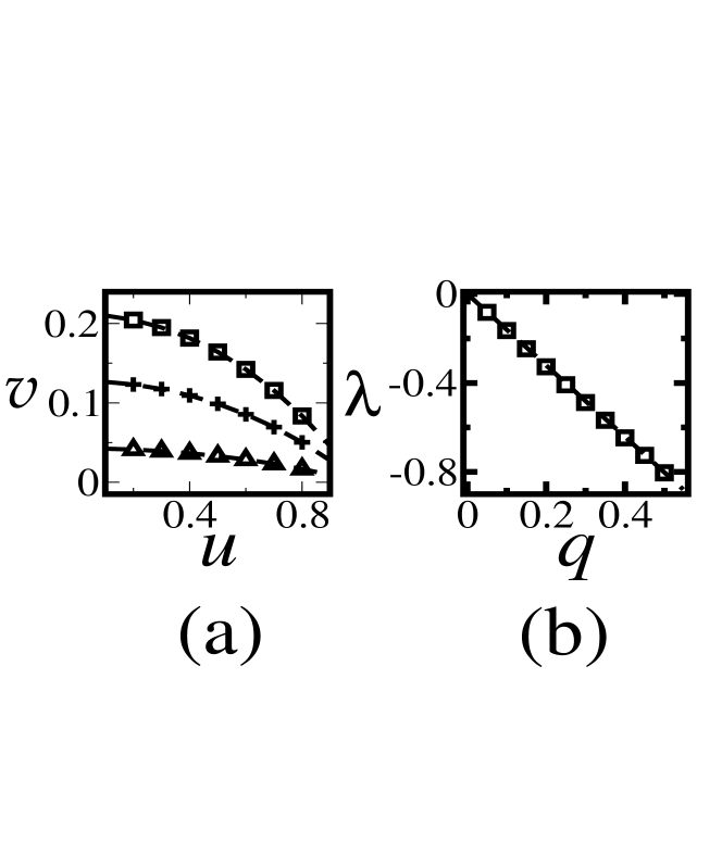
Figure 2: (a) Growth velocity $v$ as a function of inclination $u$ for the competitive model with $p=0.55$ (triangles), $p=0.65$ (crosses) and $p=0.75$ (squares). Dashed lines are parabolic fits of each set of data. (b) Estimates of $\lambda$ as a function of the reduced probability $q\equiv p-1/2$ (squares) and a least squares fit of the data (dashed line).

Fig. 2a illustrates the method to calculate $\lambda$ from the growth velocities for three different values of $p$. The parabolic fits accurately represent the data behavior for all inclinations. Using those fits and Eq. (18), we obtained estimates of $\lambda$ for each $p$. In order to check the accuracy of these estimates, we also calculated the ratio $\left(v-v_{0}\right)/u^{2}$ ($v_{0}$ is the growth velocity at zero slope), and extrapolated that ratio to the limit $u\to 0$. The estimates of $\lambda$ agreed with those obtained from the parabolic fits within error bars. In Fig. 2b we show $\lambda$ versus $q$, which confirms the linear relation between those quantities for a large range of values of $q$, in agreement with the KPZ equation obtained for the process.

III Numerical study of the EW-KPZ crossover

First we recall the arguments that lead to the prediction of a crossover exponent $\phi=4$.

In the works of Grossmmann, Guo and Grant (GGG) GGG and of Nattermann and Tang (NT) NT (see also forrest ), this result is derived from multiscaling relations for systems with crossover EW-KPZ in $d=1$. They proposed relations in the form

$$W(L,t)=L^{\alpha}f\left({\frac{t}{t_{c}},\frac{L}{\xi_{c}}}\right),$$ (19)

where $\xi_{c}\sim t_{c}^{1/z_{EW}}$ is a crossover length and $z_{EW}=2$ is the dynamical exponent of EW processes. Assuming that $t_{c}$ scales as Eq. (5), they obtained $\phi=z_{EW}/(\alpha_{EW}+z_{EW}-2)$ using scaling arguments. In $d=1$, we have $\beta_{EW}=1/4$ and $\alpha_{EW}=1/2$, which gives $\phi=4$ in $d=1$. This was confirmed by one-loop renormalization group calculations by NT.

The same result also follows from the expected roughness scaling of KPZ in $d=1$. Assuming dynamic scaling in the nonlinear and saturation regimes, Amar and Family AF ; AF2 showed that the roughness scales as

$$W(L,t)\sim L^{1/2}g\left(|\lambda|\frac{t}{L^{3/2}}\right),$$ (20)

where $g$ is a scaling function and where the dependence of $W$ on the parameters $\nu$ and $D$ of Eq. (1) was omitted. In the growth regime, it gives $W\sim{|\lambda|}^{1/3}t^{1/3}$ ($\beta_{KPZ}=1/3$ in Eq. 3). Now assuming that the crossover EW-KPZ takes place when the EW roughness (Eq. 3 with $\beta_{EW}=1/4$) matches that of KPZ, as illustrated in Fig. 1, we obtain $\lambda^{1/3}{t_{c}}^{1/3}\sim{t_{c}}^{1/4}$, from which $\phi=4$ also follows.

This last argument is the basis for the numerical calculation of $t_{c}$ using the roughness in the EW and KPZ regimes. First, it is necessary to calculate scaling amplitudes not shown in Eq. (3): for the EW regime we have

$$W_{E}\approx At^{1/4},$$ (21)

and for the KPZ regime we have

$$W_{K}\approx Bt^{1/3}.$$ (22)

Matching these forms at $t_{c}$ we obtain

$$t_{c}\approx{\left({A\over B}\right)}^{12}.$$ (23)

Consequently, $t_{c}$ can be determined from the estimates of the amplitudes $A$ and $B$.

Simulations of the RSOS model with deposition and evaporation were done for several values of $p$, in lattices with $L={10}^{5}$, up to times approximately ${10}^{6}$. $100$ deposits were generated for each $p$.

In Fig. 3 we show $W/t^{1/4}$ for small times $t$ with $p=0.7$ and $p=0.6$. That ratio is expected to be constant in the EW regime. A narrow region $20\leq t\leq 40$ with this feature is observed for $p=0.7$, while a wider EW region is found for smaller $p$. Here it is important to recall that other competitive models fail at this point because a clear EW region is found only for very small $p$, where the KPZ regime becomes difficult to be attained in simulation; one example is the model involving ballistic deposition and the Family model studied in Ref. chamereis .

The calculation of amplitude $B$ is slightly more difficult because the ratios $W/t^{1/3}$ are not constant inside a time window long enough to extend to the maximum simulation times. In other words, the presence of significant corrections to scaling in Eq. (22) has to be taken into account. This can be done with the extrapolation of $W/t^{1/3}$ as a function of $1/t^{1/3}$, as shown in Fig. 4 for $p=0.7$ and $p=0.6$ (see also Ref. chamereis ). Although the range of the variable $1/t^{1/3}$ (abscissa of Fig. 4) is relatively small, it comprises almost two decades of the largest values of $t$. Good linear fits of the data are obtained in these large time regions, which suggests constant (but large) subdominant corrections to Eq.(22). The amplitude $B$ is estimated from the intersection of those fits with the vertical axis ($t\to\infty$).

For fixed $p$, different ranges of the variable $1/t^{1/3}$ were chosen for the extrapolation of the data and the calculation of error bars in the estimates of the amplitude $B$. This procedure provides reliable and accurate final estimates of that amplitude. For instance, for $p=0.7$ (Fig. 4), we obtain $B=0.330\pm 0.004$. We also observe that, while the amplitude $A$ slowly varies with $p$ (nearly $10\%$ from $p=0.55$ to $p=0.8$), the amplitude $B$ has a remarkable dependence on $p$.

The estimates of $t_{c}$ obtained from Eq. (23) are shown in Fig. 5 as a function of $q\equiv p-1/2$. Linear fits of different subsets of those data give

$$t_{c}\sim q^{-\left(4.1\pm 0.1\right)}.$$ (24)

The linear relation between $q$ and $\lambda$ implies $\phi=4.1\pm 0.1$, which is in excellent agreement with the theoretically predicted value.

Here it is important to recall that, in other competitive models such as the RDSR-BD one chamereis , the calculation of $t_{c}$ with accuracy was not possible. For instance, a clear EW growth regime (with $\beta_{EW}=1/4$) is observed in that model only for very small $p$, but in these conditions the KPZ growth regime (with $\beta_{KPZ}=1/3$) is not attained within a reasonable simulation time. This may be a consequence of the typically huge scaling corrections of BD balfdaar . However, we believe that the main reason for those difficulties is the parabolic $\lambda-p$ relation, which significantly reduces the range of $p$ where both regimes can be numerically analyzed.

IV Conclusion

We studied a competitive growth model in $1+1$ dimensions involving RSOS deposition, with probability $p$, and RSOS evaporation, with probability $1-p$. This model may be viewed as a discrete realization of the continuum KPZ equation with an adjustable nonlinear coupling $\lambda$ related to $p$. Its corresponding KPZ equation is derived, showing that $|\lambda|$ linearly increases with $q\equiv p-1/2$, so that the process belongs to the EW class for $p=1/2$. This result is confirmed numerically by calculation of tilt-dependent velocities for several values of $p$. It contrasts to the parabolic $\lambda-p$ relation obtained for competing models involving a KPZ and an EW process, which shows that this relation, although being of wide applicability, is not universal.

We also calculated numerically the scaling amplitudes of the EW and KPZ growth regimes for several values of $p$. From these quantities, estimates of the crossover times $t_{c}$ were obtained. They scale as Eq. (5) with $\phi=4.1\pm 0.1$, in excellent agreement with the theoretically predicted value of the crossover exponent. This result improves previous ones, which suggested $\phi\approx 3$ from simulations of the KPZ equation. We believe that this work provides an important, possibly definite confirmation of scaling relations predicted for the EW-KPZ crossover in $d=1$.

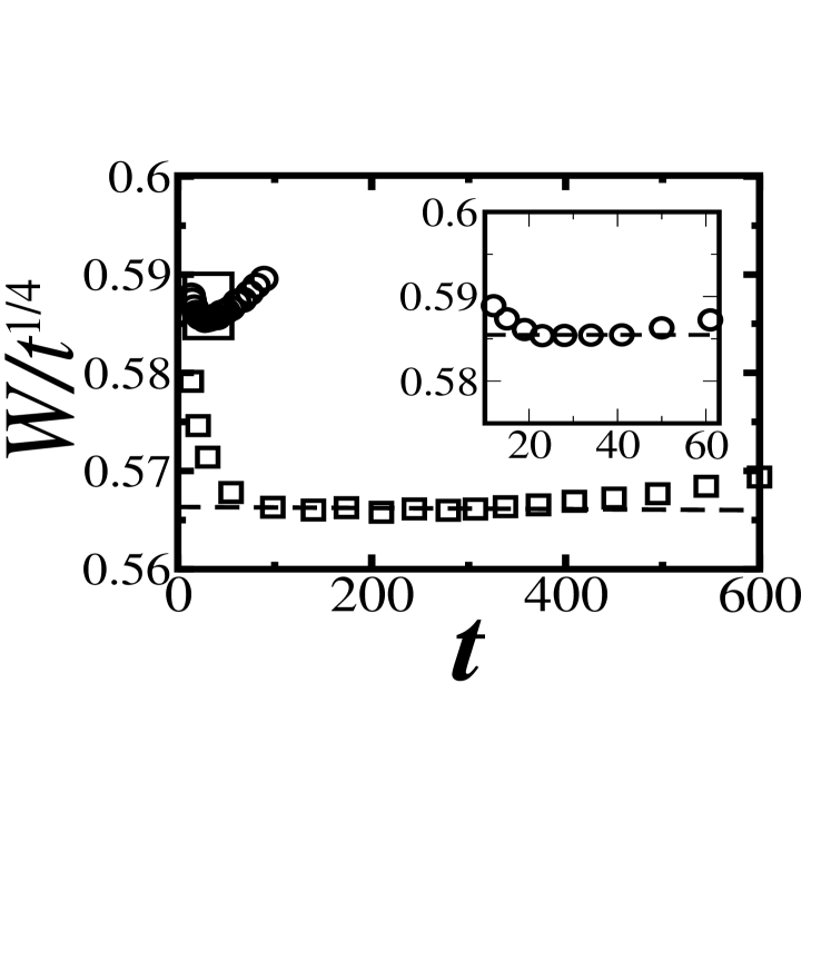
Figure 3: $W/t^{1/4}$ at small times $t$ for the competitive model with $p=0.7$ (circles) and $p=0.6$ (squares) in a large lattice ($L={10}^{5}$). The inset shows a zoom of the data for $p=0.7$ in the EW region. The dashed lines are linear fits of the data in those regions.

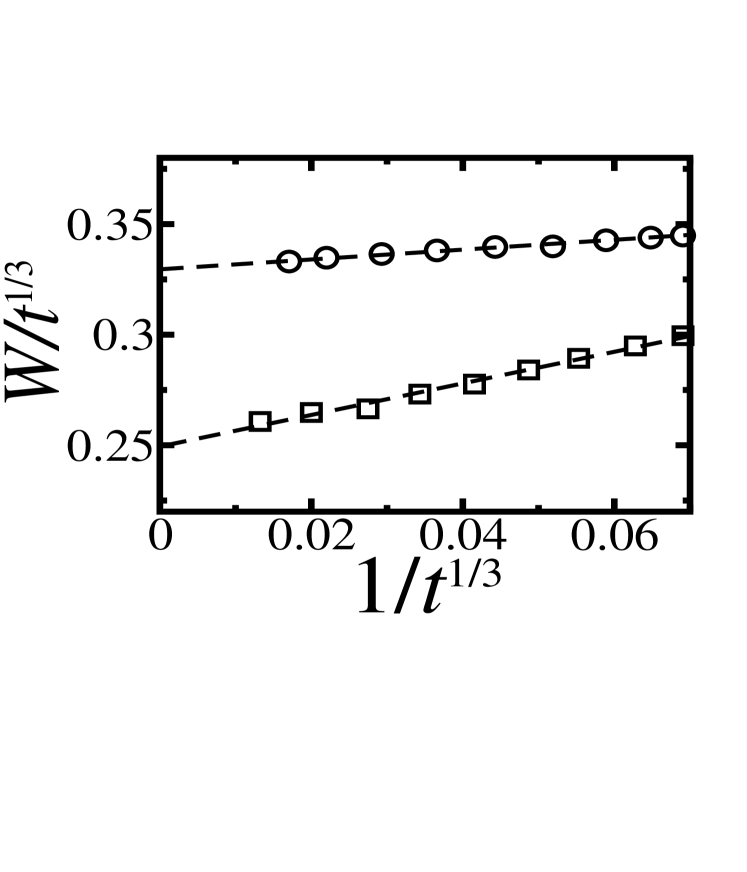
Figure 4: $W/t^{1/3}$ versus $1/t^{1/3}$ at long times, for $p=0.7$ (circles) and $p=0.6$ (squares) in a large lattice ($L={10}^{5}$). The dashed lines are linear fits of the data.

Figure 5: Crossover time $t_{c}$ versus $q\equiv p-1/2$ for the competitive model with $0.55\leq p\leq 0.8$. The dashed line is a linear fit of the plot, with slope near $-4.1$.

- (1) C. M. Horowitz, R. A. Monetti, E. V. Albano, Phys. Rev. E 63, 66132 (2001).
- (2) C. M. Horowitz and E. Albano, J. Phys. A: Math. Gen. 34 357 (2001); Eur. Phys. J. B 31, 563 (2003).
- (3) Y. Shapir, S. Raychaudhuri, D. G. Foster, and J. Jorne, Phys. Rev. Lett. 84, 3029 (2000).
- (4) Y. P. Pellegrini and R. Jullien, Phys. Rev. Lett. 64 1745 (1990); Phys. Rev. A 43 920 (1991).
- (5) T. J. da Silva and J. G. Moreira, Phys. Rev. E 63, 041601 (2001).
- (6) A. Chame and F. D. A. Aarão Reis, Phys. Rev. E 66, 051104 (2002).
- (7) D. Muraca, L. A. Braunstein, and R. C. Buceta, Phys. Rev. E 69, 065103(R) (2004).
- (8) L. A. Braunstein and C.-H. Lam, Phys. Rev. E 72, 026128 (2005).
- (9) F. D. A. Aarão Reis, Phys. Rev. E, to appear (2006).
- (10) A. Kolakowska, M. A. Novotny and P. S. Verma, Phys. Rev. E 70, 051602 (2004); cond-mat/0509668 (2005).
- (11) L. A. Bulavin, N. I. Lebovka, V. Y. Starchenko, and N. V. Vygornitskii, Physica A 328, 505 (2003).
- (12) J. Yu and J. G. Amar, Phys. Rev. E 65, 060601(R) (2002).
- (13) S. F. Edwards and D. R. Wilkinson, Proc. R. Soc. London 381 17 (1982).
- (14) M. Kardar, G. Parisi and Y.-C. Zhang, Phys. Rev. Lett. 56 889 (1986).
- (15) A. L. Barabási and H. E. Stanley, Fractal concepts in surface growth (Cambridge University Press, Cambribge, England, 1995).
- (16) J. G. Amar and F. Family, Phys. Rev. A 45 R3373 (1992).
- (17) B. Grossmann, H. Guo, and M. Grant, Phys. Rev. A 43 1727 (1991).
- (18) T. Nattermann and L.-H. Tang, Phys. Rev. A 45 7156 (1992).
- (19) B. M. Forrest and R. Toral, J. Stat. Phys. 70, 703 (1993).
- (20) M. J. Vold, J. Coll. Sci. 14 168 (1959); J. Phys. Chem. 63 1608 (1959).
- (21) F. Family, J. Phys. A 19 L441 (1986).
- (22) J. M. Kim and J. M. Kosterlitz, Phys. Rev. Lett. 62 2289 (1989).
- (23) J. G. Amar and F. Family, Phys. Rev. A 45 5378 (1992).
- (24) N. G. Van Kampen, Stochastic Processes in Physics and Chemistry (Noth-Holland, Amsterdam, 1981).
- (25) K. Park and B. N. Kahng, Phys. Rev. E, 51, 796 (1995).
- (26) C. Baggio, R. Vardavas, and D. D. Vvedensky, Phys. Rev. E 64, 045103(R) (2001); D. D. Vvedensky, Phys. Rev. E 67, 025102(R) (2003).
- (27) D. D. Vvedensky, Phys. Rev. E 68, 010601 (2003).
- (28) B. Derrida and K. Mallick, J. Phys. A: Math. Gen. 30, 1031 (1997).
- (29) J. Krug and P. Meakin, J. Phys. A: Math. Gen. 23 L987 (1990).
- (30) J. Krug and H. Spohn, Phys. Rev. Lett. 64, 2332 (1990).
- (31) D. A. Huse, J. G. Amar, and F. Family, Phys. Rev. A 41, 7075 (1990).
- (32) F. D. A. Aarão Reis, Phys. Rev. E 63, 056116 (2001); Phys. Rev. E 69 021610 (2004).