Dynamical mean-field theory using Wannier functions:
a flexible route to electronic structure calculations of strongly correlated materials

Abstract

A versatile method for combining density functional theory (DFT) in the local density approximation (LDA) with dynamical mean-field theory (DMFT) is presented. Starting from a general basis-independent formulation, we use Wannier functions as an interface between the two theories. These functions are used for the physical purpose of identifying the correlated orbitals in a specific material, and also for the more technical purpose of interfacing DMFT with different kinds of band-structure methods (with three different techniques being used in the present work). We explore and compare two distinct Wannier schemes, namely the maximally-localized-Wannier-function (MLWF) and the $N$-th order muffin-tin-orbital (NMTO) methods. Two correlated materials with different degrees of structural and electronic complexity, SrVO₃ and BaVS₃, are investigated as case studies. SrVO₃ belongs to the canonical class of correlated transition-metal oxides, and is chosen here as a test case in view of its simple structure and physical properties. In contrast, the sulfide BaVS₃ is known for its rich and complex physics, associated with strong correlation effects and low-dimensional characteristics. New insights into the physics associated with the metal-insulator transition of this compound are provided, particularly regarding correlation-induced modifications of its Fermi surface. Additionally, the necessary formalism for implementing self-consistency over the electronic charge density in a Wannier basis is discussed.

I Introduction

One of the fundamental points that underlies the rich physics of strongly correlated electron systems is the competition between the electrons tendency to localize, and their tendency to delocalize by forming quasiparticle (QP) bands. Traditional effective single-particle (i.e. band-structure) theories emphasize the latter aspect, which is appropriate when the kinetic energy dominates. For such materials, computational techniques based on electronic density functional theory (DFT) (see e.g. Refs. [Kohn, 1999; Jones and Gunnarsson, 1989] for reviews) have nowadays reached a very high degree of accuracy and yield remarkable agreement with experiment.

In correlated materials however, the screened Coulomb interaction is a major aspect of the problem, which cannot be treated perturbatively, and independent-particle descriptions fail. Albeit the representability of the electronic charge density by a set of Kohn-Sham Kohn and Sham (1965) (KS) orbitals is still guaranteed in most cases, this raises the question of whether such a representation is physically appropriate. Furthermore, the description of excited states of the many-particle system must be based on other observables than just the charge density, such as the energy-dependent spectral function. Any appropriate theoretical framework must then treat band formation (best described in momentum space) and the tendency to localization (best described in real space) on an equal footing. For this reason, there is an increasing awareness that many-body descriptions must also include real-space, orbitally resolved, descriptions of the solid, close to the quantum chemistry of the material under consideration Perdew and Schmidt (2001); Krieger and Iafrate (1992). In correlated metals, the coexistence of coherent QP bands at low energy with high-energy incoherent Hubbard bands (which originate from atomic-like transitions persisting in the solid state) is a vivid demonstration that a dual description (both in momentum space and in real space) is needed. Such a dual description is at the heart of dynamical mean-field theory (DMFT) (see e.g. Refs. [Georges et al., 1996; Georges, 2004; Held et al., 2002; Biermann, 2006; Kotliar and Vollhardt, 2004; Kotliar et al., 2006] for reviews), which in recent years has proven to be a tool of choice for treating strong-correlation effects. This theory has been successfully combined with electronic-structure methods within the framework of the local density approximation Kohn and Sham (1965) (LDA) to DFT Anisimov et al. (1997); Lichtenstein and Katsnelson (1998) (also labeled as LDA+DMFT), or so-called GW formalisms Biermann et al. (2003a, b); Kotliar and Savrasov (2001).

A central physical issue in merging the momentum-space and local descriptions within those many-body approaches is the identification of a subspace of orbitals in which correlations are treated using non-perturbative many-body techniques. Furthermore, an important technical issue is the choice of a convenient basis set for interfacing the many-body and the band-structure parts of the calculation. Because the original Wannier construction Wannier (1937) is based on a decomposition of the extended Bloch states into a superposition of rather localized orbitals, it appears that appropriate generalizations of this construction leading to well-localized basis functions should provide an appropriate framework for many-body calculations. Exploring this in detail is the main purpose of this paper. In fact, there has been recently a growing activity associated with the Wannier formalism in the context of many-body approaches. The use of Wannier basis sets in the LDA+DMFT context has been lately pioneered by several groups, using either the $N$-th order muffin-tin orbital (NMTO) framework Pavarini et al. (2004); Poteryaev et al. (2004); Biermann et al. (2005); Pavarini et al. (2005) or other types of Wannier constructions based on the linear muffin-tin orbital (LMTO) framework Anisimov et al. (2005); Gavrichkov et al. (2005); Solovyev (2006); Anisimov et al. (2006). For a detailed presentation of such implementations see Ref. [Anisimov et al., 2005]. Furthermore, the computation of many-body interaction parameters has also been discussed Ku et al. (2002); Schnell et al. (2003).

In this context, the main motivations of the present article are the following:

• We give a presentation of the LDA+DMFT formalism in a way which should make it easier to interface it with a band-structure method of choice. To this aim, we are careful to distinguish between two key concepts: the orbitals defining the correlated subspace in which a many-body treatment is done, and the specific basis set which is used in order to interface the calculation with a specific band-structure method. The LDA+DMFT approach is first presented in a manner which makes no reference to a specific basis set, and then only some technical issues associated with choosing the basis set for implementation are discussed.

• It is explained how the Wannier-functions formalism provides an elegant solution to both the physical problem of identifying the correlated orbitals and to the more technical issue of interfacing DMFT with basically any kind of band-structure method. So far the LDA+DMFT technique has been implemented with band-structure codes based on muffin-tin-orbital (MTO)-like representations Andersen (1975). Although this realization is very successful, we feel that broadening the range of band-structure methods that can be used in the LDA+DMFT context may make this method accessible to a larger part of the band-structure community, hence triggering further progress on a larger scale. As an example, one could think of problems involving local structural relaxations, which are more difficult to handle within the MTO formalism than in plane-wave like approaches.

• In this work, two different Wannier constructions are applied and the corresponding results are compared in detail. Though there are numerous ways of constructing Wannier(-like) functions we have chosen such methods that derive such functions in a post-processing step from a DFT calculation. In this way the method is, at least in principle, independent of the underlying band-structure code and therefore widely accessible. First, we used the maximally-localized-Wannier-functions (MLWFs) method proposed by Marzari, Vanderbilt and Souza Marzari and Vanderbilt (1997); Souza et al. (2001). Second, we constructed Wannier functions using the $N$-th order MTO (NMTO) framework following Andersen and coworkers Andersen and Saha-Dasgupta (2000); Andersen et al. (2000); Zurek et al. (2005) which has first been used in the LDA+DMFT context in Ref. [Pavarini et al., 2004] and actively used since then (e.g. Refs. [Saha-Dasgupta et al., 2005; Pavarini et al., 2005; Nekrasov et al., 2006; Yamasaki et al., 2006a]). Note that the NMTO method also works in principle with any given, not necessarily MTO-determined, KS effective potential. However, in practice, this construction is presently only available in an MTO environment.

• We also consider the issue of fully self-consistent calculations in which many-body effects are taken into account in the computation of the electronic charge density. Appendix A is devoted to a technical discussion of implementing charge self-consistency, with special attention to the use of Wannier basis sets also in this context. However, the practical implementation of charge self-consistency in non-MTO based codes is ongoing work, to be discussed in detail in a future publication.

Two materials with correlated $3d$ electrons serve as testing grounds for the methods developed in this paper, namely the transition-metal oxide SrVO₃ and the sulfide BaVS₃. Nominally, both compounds belong to the class of $3d^{1}$ systems, where due to crystal-field splitting the single $d$ electron is expected to occupy the $t_{2g}$ states only. The latter form partially filled bands in an LDA description. The two compounds have very different physics and exhibit different degrees of complexity in their electronic structure. The metallic perovskite SrVO₃ has perfect cubic symmetry over the temperature regime of interest and displays isolated $t_{2g}$-like bands at the Fermi level, well-separated from bands higher and lower in energy. Its physical properties suggest that it is in a regime of intermediate strength of correlations. Many experimental results are available for this material (for a detailed list see Sec. III.1.1) and it has also been thoroughly investigated theoretically in the LDA+DMFT framework Liebsch (2003); Sekiyama et al. (2004); Pavarini et al. (2004, 2005); Nekrasov et al. (2005); Solovyev (2006); Nekrasov et al. (2006). For all these reasons, SrVO₃ is an ideal test case for methodological developments.

In contrast, BaVS₃ is much more complex in both its electronic structure and physical properties. The sulfide displays several second-order transitions with decreasing temperature, including a metal-insulator transition (MIT) at $\sim$70 K. Additionally, the low-energy LDA bands with strong $t_{2g}$ orbital character are entangled with other bands, mainly of dominant sulfur character, which renders a Wannier construction more challenging. In this paper, the Wannier-based formalism is used for BaVS₃ to investigate correlation-induced changes in orbital populations, and most notably, correlation-induced changes in the shape of the different Fermi-surface sheets in the metallic regime above the MIT. In the end, these changes are key to a satisfactory description of the MIT.

This article is organized as follows. Section II introduces the general theoretical formalism. First, the LDA+DMFT approach is briefly reviewed in a way which does not emphasize a specific basis set. Then, the issue of choosing a basis set for implementation and interfacing DMFT with a specific band-structure method is discussed. Finally, the Wannier construction is shown to provide an elegant solution for both picking the correlated orbitals and practical implementation. The different Wannier constructions used in this paper are briefly described, followed by some remarks on the calculational schemes employed in this work. In Sect. III the results for SrVO₃ and BaVS₃ are presented. To this aim we discuss separately the LDA band structure, the corresponding Wannier basis sets and the respective LDA+DMFT results. Appendices are devoted to the basic formalism required to implement self-consistency over the charge density and total energy calculations, as well as further technical details on the DFT calculations.

II Theoretical framework

II.1 Dynamical mean-field theory and electronic structure

II.1.1 Projection onto localized orbitals

Dynamical mean-field theory provides a general framework for electronic structure calculations of strongly correlated materials. A main concept in this approach is a projection onto a set of spatially localized single-particle orbitals $\{|\chi_{\mathbf{R}m}\rangle\}$, where the vector $\mathbf{R}$ labels a site in the (generally multi-atom) unit cell and $m$ denotes the orbital degree of freedom. These orbitals generate a subspace of the total Hilbert space, in which many-body effects will be treated in a non-perturbative manner. In the following, we shall therefore refer to this subspace as the “correlated subspace” $\mathcal{C}$, and often make use of the projection operator onto this correlated subspace, defined as:

$$\hat{P}^{(\mathcal{C})}_{\mathbf{R}}\equiv\sum_{m\in\mathcal{C}}|\chi_{\mathbf{R}m}\rangle\langle\chi_{\mathbf{R}m}|\,.$$ (1)

For simplicity, we restrict the present discussion to the basic version of DMFT in which only a single correlated site is included in this projection. In cluster generalizations of DMFT, a group of sites is taken into account. Also, it may be envisioned to generalize the method in such a way that $\mathbf{R}$ could stand for other physically designated real-space entities (e.g. a bond, etc.).

Because the many-body problem is considered in this projected subspace only, and because it is solved there in an approximate (though non-perturbative) manner, different choices of these orbitals will in general lead to different results. How to properly choose these orbitals is therefore a key question. Ultimately, one might consider a variational principle which dictates an optimal choice (cf. Appendix B). At the present stage however, the guiding principles are usually physical intuition based on the quantum chemistry of the investigated material, as well as practical considerations. Many early implementations of the LDA+DMFT approach have used a linear muffin-tin orbital Andersen (1975) (LMTO) basis for the correlated orbitals (e.g. Refs. [Lichtenstein and Katsnelson, 1998; Biermann et al., 2004]). This is very natural since in this framework it is easy to select the correlated subspace $\mathcal{C}$ regarding the orbital character of the basis functions: e.g., $d$ character in a transition-metal oxide, $f$ character in rare-earth materials, etc.. The index $m$ then runs over the symmetry-adapted basis functions (or possibly the “heads” of these LMTOs) corresponding to this selected orbital character. Exploring other choices based on different Wannier constructions is the purpose of the present paper. In this context, the index $m$ should be understood as a mere label of the orbitals spanning the correlated subset. For simplicity, we shall assume in the following that the correlated orbitals form an orthonormal set: $\langle\chi_{\mathbf{R}m}^{\hfill}|\chi_{\mathbf{R}^{\prime}m^{\prime}}^{\hfill}\rangle$=$\delta_{\mathbf{R}\mathbf{R}^{\prime}}\delta_{mm^{\prime}}$. This may not be an optimal choice for the DMFT approximation however, which is better when interactions are more local. Generalization to non-orthogonal sets is yet straightforward by introducing an overlap matrix (see e.g. Ref. [Kotliar et al., 2006]).

II.1.2 Local observables

There are two central observables in the LDA+DMFT approach to electronic structure. The first, as in DFT, is the total electronic charge density $\rho(\mathbf{r})$. The second is the local one-particle Green’s function $\mathbf{G}_{\rm{loc}}(i\omega_{n})$ projected onto $\mathcal{C}$, with components $G_{\mathbf{R}m,\mathbf{R}m^{\prime}}(i\omega_{n})$. Both quantities are related to the full Green’s function of the solid $G(\mathbf{r},\mathbf{r}^{\prime};i\omega_{n})$ by:

$$\rho(\mathbf{r}) = \frac{1}{\beta}\sum_{n}G(\mathbf{r},\mathbf{r};i\omega_{n})\,\mbox{e}^{i\omega_{n}0^{+}}$$ (2)

$$G_{mm^{\prime}}^{\rm{loc}}(i\omega_{n}) = \iint d\mathbf{r}d\mathbf{r}^{\prime}\chi_{\mathbf{R}m}^{*}(\mbox{$\mathbf{r}$$-$$\mathbf{R}$})\chi_{\mathbf{R}m^{\prime}}^{\hfill}(\mbox{$\mathbf{r}^{\prime}$$-$$\mathbf{R}$})\,G(\mathbf{r},\mathbf{r}^{\prime};i\omega_{n})\,.$$

The last expression can be abbreviated as a projection of the full Green’s function operator $\hat{G}$ according to

$$\hat{G}_{\rm{loc}}=\hat{P}_{\mathbf{R}}^{(\mathcal{C})}\,\hat{G}\,\hat{P}_{\mathbf{R}}^{(\mathcal{C})}\,.$$ (3)

In these expressions, we have used (for convenience) the Matsubara finite-temperature formalism, with $\omega_{n}$=$(2n+1)\pi/\beta$ and $\beta$=$1/k_{\rm{B}}T$. The Matsubara frequencies are related via Fourier transformation to the imaginary times $\tau$. Note that the factor e${}^{i\omega_{n}0^{+}}$ in (2) ensures the convergence of the Matsubara sum which otherwise falls of as $1/\omega_{n}$. We have assumed, for simplicity, that there is only one inequivalent correlated atom in the unit cell, so that $\hat{G}_{\rm{loc}}$ does not carry an atom index (generalization is straightforward). In the following we will drop the index $\mathbf{R}$ if not explicitly needed.

Taking the KS Green’s function $\hat{G}_{\rm{KS}}$ as a reference, the full Green’s function of the solid can be written in operator form, as: $\hat{G}^{-1}$=$\hat{G}^{-1}_{\rm{KS}}-\Delta\hat{\Sigma}$, or more explicitly (atomic units are used throughout this paper):

$$G(\mathbf{r},\mathbf{r}^{\prime};i\omega_{n})=\left\langle\mathbf{r}\left|\left[i\omega_{n}+\mu+\frac{\nabla^{2}}{2}-\hat{V}_{\rm{KS}}-\Delta\hat{\Sigma}\right]^{-1}\right|\mathbf{r}^{\prime}\right\rangle\,.$$ (4)

Here $\mu$ is the chemical potential and $V_{\rm{KS}}$ the KS effective potential, which reads:

$$V_{\rm{KS}}(\mathbf{r}) = -\sum_{i}\frac{Q_{i}}{|\mathbf{r}-\mathbf{N}_{i}|}+\int d\mathbf{r}^{\prime}\frac{\rho(\mathbf{r}^{\prime})}{|\mathbf{r}-\mathbf{r}^{\prime}|}+\frac{\delta E_{\rm{xc}}}{\delta\rho(\mathbf{r})}$$ (5)

$$= V_{\rm{ext}}(\mathbf{r})+V_{\rm{H}}(\mathbf{r})+V_{\rm{xc}}(\mathbf{r})\,,$$

where $Q$, $\mathbf{N}$ are the charges, lattice vectors of the atomic nuclei, $i$ runs over the lattice sites, $V_{\rm{ext}}$ is the external potential due to the nuclei, $V_{\rm{H}}$ denotes the Hartree potential and $V_{\rm{xc}}$ is the exchange-correlation potential, obtained from a functional derivative of the exchange-correlation energy $E_{\rm{xc}}$. For the latter, the LDA (or generalized-gradient approximations) may be used. Recall that $V_{\rm{KS}}(\mathbf{r})$ is determined by the true self-consistent electronic charge density given by Eq. (2) (which is modified by correlation effects, and hence differs in general from its LDA value, see below).

The operator$\Delta\hat{\Sigma}$ in Eq. (4) describes a many-body (frequency-dependent) self-energy correction. In the DMFT approach, this self-energy correction is constructed in two steps. First, $\mathbf{\Delta\Sigma}$ is derived from an effective local problem Georges and Kotliar (1992) (or “effective quantum impurity model”) within the correlated subspace $\mathcal{C}$ via:

$$\Delta\Sigma_{mm^{\prime}}(i\omega_{n})\equiv\Sigma^{\rm{imp}}_{mm^{\prime}}(i\omega_{n})-\Sigma^{\rm{dc}}_{mm^{\prime}}\,,$$ (6)

whereby $\mathbf{\Sigma}_{\rm{dc}}$ is a double-counting term that corrects for correlation effects already included in conventional DFT. The self-energy correction to be used in (4), and subsequently in (12,13), is then obtained by promoting (6) to the lattice, i.e.,

$$\Delta\Sigma(\mathbf{r},\mathbf{r}^{\prime};i\omega_{n})\equiv$$

$$\sum_{\mathbf{T}mm^{\prime}}\chi^{*}_{m}(\mbox{$\mathbf{r}$$-$$\mathbf{R}$$-$$\mathbf{T}$})\chi_{m^{\prime}}^{\hfill}(\mbox{$\mathbf{r}^{\prime}$$-$$\mathbf{R}$$-$$\mathbf{T}$})\,\Delta\Sigma_{mm^{\prime}}(i\omega_{n})\,,$$ (7)

where $\mathbf{T}$ denotes a direct lattice vector. The key approximation is that the self-energy correction is non-zero only inside the (lattice-translated) correlated subspace, i.e., $\Delta\hat{\Sigma}$=$\Delta\hat{\Sigma}^{(\mathcal{C})}$, hence exhibits only on-site components in the chosen orbital set.

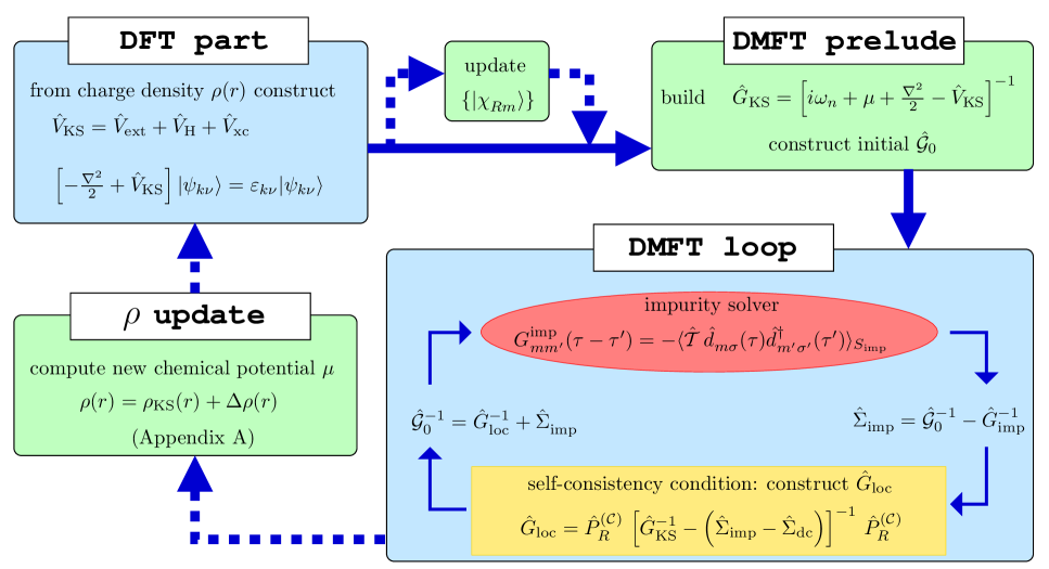
Figure 1: Complete self-consistency loop for LDA+DMFT. The charge density $\rho$ determines the KS potential $V_{\rm{KS}}$, from which KS eigenvalues $\varepsilon_{\mathbf{k}\nu}$ and eigenfunctions $\psi^{\hfill}_{{\mathbf{k}}\nu}$ follow. The KS Green’s function is then constructed and passed on to the DMFT cycle (in practice, the KS Hamiltonian $\mathbf{H}_{\rm{KS}}$ is constructed in the basis set used to implement the method, and transferred to the DMFT cycle). The DMFT loop consists in i) solving the effective impurity problem for the impurity Green’s function, hence obtaining an impurity self-energy, ii) combining the self-energy correction with the KS Green’s function in order to obtain the local Green’s function $\mathbf{G}_{\rm{loc}}$ projected in the correlated subset and iii) obtaining an updated Weiss mean-field. An initial guess for the Weiss dynamical mean-field must be made at the beginning of the DMFT loop, e.g. by choosing $\hat{{\cal G}}_{0}^{\rm{init}}=\hat{P}^{(\mathcal{C})}\hat{G}_{\rm{KS}}\hat{P}^{(\mathcal{C})}$. Is the DMFT loop converged, the chemical potential is updated in order to ensure global charge neutrality, and the new charge density (including many-body effects) is constructed (described in Appendix. A). This new density determines a new KS potential. Note that in addition one may want to update the set $\{|\chi_{m}^{\hfill}\rangle\}$ when preparing for the next DMFT loop (cf. Appendix B). The whole process must be iterated until the charge density, the impurity self-energy and the chemical potential are converged. In practice, good convergence of the DMFT loop is reached before a new $\rho$ is calculated. Note that in the present paper using a Wannier implementation, the global self-consistency on the charge density is not implemented in practice. Thus the self-consistent LDA Hamiltonian $\mathbf{H}_{\rm{KS}}$ enters the DMFT loop, which is iterated until convergence of the self-energy.

II.1.3 Effective quantum impurity problem

The local impurity problem can be viewed as an effective atom involving the correlated orbitals, coupled to a self-consistent energy-dependent bath. It can be formulated either in Hamiltonian form, by explicitly introducing the degrees of freedom of the effective bath, or as an effective action in which the bath degrees of freedom have been integrated out. In the latter formulation, the action of the effective impurity model reads:

$$S_{\rm{imp}}=-\iint_{0}^{\beta}d\tau d\tau^{\prime}\sum_{mm^{\prime}\sigma}d^{\dagger}_{m\sigma}(\tau)[\mathcal{G}_{0}^{-1}]_{mm^{\prime}}(\tau-\tau^{\prime})d^{\hfill}_{m^{\prime}\sigma}(\tau^{\prime})$$

$$\hskip 28.45274pt+\int_{0}^{\beta}d\tau\,H_{U}\left(\{d^{\dagger}_{m\sigma};d_{m\sigma}\}\right)\quad.$$ (8)

In this expression, $d^{\dagger}_{m\sigma}$, $d^{\hfill}_{m\sigma}$ are the Grassmann variables corresponding to orbital $\chi^{\hfill}_{m}$ for spin $\sigma$, $\hat{H}_{U}$ is a many-body interaction (to be discussed in section II.3.2), and $\hat{\mathcal{G}}_{0}(i\omega_{n})$ is the dynamical mean-field, determined self-consistently (see below), which encodes the coupling of the embedded atom to the effective bath. This quantity is the natural generalization to quantum many-body problems of the Weiss mean-field of classical statistical mechanics. Its frequency dependence is the essential feature which renders DMFT distinct from static approaches such as e.g. the LDA+U method Anisimov et al. (1991). The frequency dependence allows for the inlcusion of all (local) quantum fluctuations. Thereby the relevant (possibly multiple) energy scales are properly taken into account, as well as the description of the transfers of spectral weight. One should note that the dynamical mean-field $\hat{\mathcal{G}}_{0}(i\omega_{n})$ formally appears as the bare propagator in the definition of the effective action for the impurity (8). However, its actual value is only known after iteration of a self-consistency cycle (detailed below) and hence depends on many-body effects for the material under consideration.

The self-energy correction is obtained from the impurity model as:

$$\mathbf{\Sigma}_{\rm{imp}}(i\omega_{n})\equiv\mbox{\boldmath$\mathcal{G}$\unboldmath}_{0}^{-1}(i\omega_{n})-\mathbf{G}_{\rm{imp}}^{-1}(i\omega_{n})\quad.$$ (9)

in which $\mathbf{G}_{\rm{imp}}$ is the impurity model Green’s function, associated with the effective action (8) and defined as:

$$G^{\rm{imp}}_{mm^{\prime}}(\tau-\tau^{\prime})\equiv-\langle\hat{\mathcal{T}}\,\hat{d}^{\hfill}_{m\sigma}(\tau)\hat{d}^{\dagger}_{m^{\prime}\sigma^{\prime}}(\tau^{\prime})\rangle_{S_{\rm{imp}}}\quad,$$ (10)

where $\mathcal{T}$ stands for time-ordering. Note that computing this Green’s function, given a specific Weiss dynamical mean-field $\hat{\mathcal{G}}_{0}(i\omega_{n})$ is in fact the most demanding step in the solution of the DMFT equations.

II.1.4 Self-consistency conditions

In order to have a full set of self-consistent equations, one still needs to relate the effective impurity problem to the whole solid. Obviously, the dynamical mean-field $\mathcal{G}$${}_{0}(i\omega_{n})$ is the relevant link, but we have not yet specified how to determine it. The central point in DMFT is to evaluate $\mathcal{G}$${}_{0}(i\omega_{n})$ in a self-consistent manner by requesting that the impurity Green’s function coincides with the components of the lattice Green’s function projected onto the correlated subspace $\mathcal{C}$, namely that:

$$\mathbf{G}_{\rm{imp}}=\mathbf{G}_{\rm{loc}}\quad,$$ (11)

or, in explicit form, using (2,4,6) and (7):

$$G^{\rm{imp}}_{mm^{\prime}}(i\omega_{n})=\iint d\mathbf{r}d\mathbf{r}^{\prime}\chi_{m}^{*}(\mbox{$\mathbf{r}$$-$$\mathbf{R}$})\chi_{m^{\prime}}^{\hfill}(\mbox{$\mathbf{r}^{\prime}$$-$$\mathbf{R}$})\times$$ (12)

$$\times\left\langle\mathbf{r}\left|\left[i\omega_{n}+\mu+\frac{\nabla^{2}}{2}-\hat{V}_{\rm{KS}}-\left(\hat{\Sigma}_{\rm{imp}}-\hat{\Sigma}_{\rm{dc}}\right)\right]^{-1}\right|\mathbf{r}^{\prime}\right\rangle\,.$$

In this representation, it is clear that the self-consistency condition involves only impurity quantities, and therefore yields a relation between the dynamical mean-field $\hat{{\cal G}}_{0}$ and $\hat{G}_{\rm{imp}}$ which, together with the solution of the impurity problem Eqs. (8-10) fully determines both quantities in a self-consistent way.

The effective impurity problem (8) can in fact be thought of as a reference system allowing one to represent the local Green’s function. This notion of a reference system is analogous to the KS construction, in which the charge density is represented as the solution of a single-electron problem in an effective potential (with the difference that here, the reference system is an interacting one).

Finally, by combining (2) and (4) the electronic charge density is related to the KS potential by:

$$\rho(\mathbf{r})=\frac{1}{\beta}\sum_{n}\left\langle\mathbf{r}\left|\left[i\omega_{n}+\mu+\frac{\nabla^{2}}{2}-\hat{V}_{\rm{KS}}-\Delta\hat{\Sigma}\right]^{-1}\right|\mathbf{r}\right\rangle\,\mbox{e}^{i\omega_{n}0^{+}}\,,$$ (13)

Expression (13) calls for two remarks. Firstly, many-body effects in $\mathcal{C}$ affect via $\mathbf{\Delta\Sigma}$ the determination of the charge density, which will thus differ at self-consistency from its LDA value. Secondly, the familiar KS representation of $\rho(\mathbf{r})$ in terms of virtually independent electrons in an effective static potential is modified in LDA+DMFT in favor of a non-local and energy-dependent (retarded) potential given by $V_{\rm{KS}}(\mathbf{r})\delta(\mathbf{r}-~{}\mathbf{r}^{\prime})\delta(\tau-\tau^{\prime})+\Delta\Sigma(\mathbf{r},\mathbf{r}^{\prime};\tau-\tau^{\prime})$. In Appendix A, we give a more detailed discussion of the technical aspects involved in calculating the charge density from expression (13). However, we have not yet implemented this calculation in practice in our Wannier-based code: the computations presented in this paper are performed for the converged $\rho(\mathbf{r})$ obtained at the LDA level. Finally, let us mention that the LDA+DMFT formalism and equations presented above can be derived from a (free-energy) functional Savrasov and Kotliar (2004) of both the charge density and the projected local Green’s function, $\Gamma[\rho,\mathbf{G}_{\rm{loc}}]$. This is reviewed in Appendix B, where the corresponding formula for the total energy is also discussed.

Fig. 1 gives a synthetic overview of the key steps involved in performing a fully self-consistent LDA+DMFT calculation, irrespective of the specific basis set and band-structure code chosen to implement the method.

II.1.5 Double-counting correction

We briefly want to comment on the double-counting (DC) correction term. Since electronic correlations are already partially taken into account within the DFT approach through the LDA/GGA exchange-correlation potential, the double-counting correction $\mathbf{\Sigma}_{\rm{dc}}$ has to correct for this in LDA+DMFT. The problem of precisely defining DC is hard to solve in the framework of conventional DFT Czy$\dot{\text{z}}$yk and Sawatzky (1994); Petukhov et al. (2003). Indeed, DFT is not an orbitally-resolved theory and furthermore the LDA/GGA does not have a diagrammatic interpretation (like simple Hartree-Fock) which would allow to subtract the corresponding terms from the DMFT many-body correction. Simply substracting the matrix elements of $V_{\rm{H}}$ and $V_{\rm{xc}}$ in the correlated orbital subset $\mathcal{C}$ from the KS Green’s function to which the many-body self-energy is applied to is not a physically reasonable strategy. Indeed, the DMFT approach (with a static, frequency-independent Hubbard interaction) is meant to treat the low-energy, screened interaction, so that the Hartree approximation is not an appropriate starting point. Instead, one wants to benefit from the spatially-resolved screening effects which are already partially captured at the LDA level. In practice, the DC terms introduced for LDA+U, i.e., “fully-localized limit” Anisimov et al. (1993) and “around mean field” Anisimov et al. (1991); Czy$\dot{\text{z}}$yk and Sawatzky (1994), appear to be reasonable also in the LDA+DMFT framework. It was recently shown Anisimov et al. (2006), that the fully-localized-limit form can be derived from the demand for discontinuity of the DFT exchange-correlation potential at integer filling.

The DC issue in fact has a better chance to be resolved in a satisfactory manner, from both the physical and formal points of view, when the concept of local interaction parameters is extended to frequency-dependent quantities (e.g. a frequency-dependent Hubbard interaction $U(\omega)$), varying from the bare unscreened value at high frequency to a screened value at low energy, and determined from first principles. The GW+DMFT construction, and the extended DMFT framework, in which this quantity plays a central role and is determined self-consistently on the same footing as the one-particle dynamical mean field, may prove to be a fruitful approach in this respect.

II.1.6 Implementation: choice of basis sets and Hilbert spaces

In the previous sections, care has been taken to write the basic equations of the LDA+DMFT formalism in a basis-independent manner. In this section, we express these equations in a general basis set, which is essential for practical implementations, and discuss advantages and drawbacks of different choices for the basis set. At this point, a word of caution is in order: it is important to clearly distinguish between the set of local orbitals $\{|\chi_{m}\rangle\}$ which specifies the correlated subspace, and the basis functions which one will have to use in order to implement the method in practice within a electronic-structure code. Different choices for $\{|\chi_{m}\rangle\}$ will lead to different results, since DMFT involves a local approximation which has a different degree of accuracy in diverse orbital sets. In contrast, once the correlated orbital set is fixed, any choice of basis set can be used in order to implement the method, with in principle identical results.

Let us denote a general basis set by $\{|B_{{\bf k}\alpha}\rangle\}$, in which ${\bf k}$ runs over the Brillouin zone (BZ) and $\alpha$ is a label for the basis functions. For example if the KS (Bloch) wave functions are used as a basis set, $\alpha$=$\nu$ is a band index and the basis functions are $\psi_{\mathbf{k}\nu}(\mathbf{r})$=e${}^{i{\bf k}.\mathbf{r}}u_{\mathbf{k}\nu}(\mathbf{r})$. In the case of a pure plane-wave basis set, $\alpha$=$\mathbf{G}$ runs over reciprocal lattice vectors. For a Bloch sum of LMTOs $\alpha$=$(\mathbf{R}lm)$ runs over sites in the primitive cell and orbital (angular momentum) quantum number. For hybrid basis sets one may have $\alpha$=$(\mathbf{R}lm,\mathbf{G})$. As an example for the latter serves the linear augmented-plane-wave Andersen (1975) (LAPW) basis set, though here in the end it is summed over the orbital indices and the basis is finally labelled by $\mathbf{G}$ only.

Consider now the DMFT self-consistency condition (11). In the (yet arbitrary) basis set $\{|B_{{\bf k}\alpha}\rangle\}$, its explicit expression in reciprocal space reads (correct normalization of the $k$-sum is understood):

$$G^{\rm{imp}}_{mm^{\prime}}(i\omega_{n}) = \sum_{\mathbf{k}}\sum_{\alpha\alpha^{\prime}}\langle\chi_{m}^{\mathbf{k}}|B_{{\bf k}\alpha}\rangle\langle B_{{\bf k}\alpha^{\prime}}|\chi_{m^{\prime}}^{\mathbf{k}}\rangle\times$$ (14)

$$\times\left\{\left[i\omega_{n}+\mu-\mathbf{H}_{\rm{KS}}(\mathbf{k})-\mathbf{\Delta\Sigma}(\mathbf{k},i\omega_{n})\right]^{-1}\right\}_{\alpha\alpha^{\prime}}\,,$$

where $|\chi_{m}^{\mathbf{k}}\rangle$= $\sum_{\mathbf{T}}\mbox{e}^{i\mathbf{k}\cdot(\mathbf{T}+\mathbf{R})}|\chi_{m}^{\hfill}\rangle$ denotes the Bloch transform of the local orbitals. In this expression, $\mathbf{H}_{\rm{KS}}(\mathbf{k})$ is the KS Hamiltonian at a given $k$-point, expressed in the basis set of interest:

$$\hat{H}_{\rm{KS}}(\mathbf{k})=\sum_{\alpha\alpha^{\prime}}|B_{{\bf k}\alpha}\rangle\langle B_{{\bf k}\alpha^{\prime}}|\left[\sum_{\nu}\varepsilon_{\mathbf{k}\nu}\langle B_{{\bf k}\alpha}|\psi_{\mathbf{k}\nu}\rangle\langle\psi_{\mathbf{k}\nu}|B_{{\bf k}\alpha^{\prime}}\rangle\right]\,,$$ (15)

with $\{\varepsilon_{\mathbf{k}\nu},\psi_{\mathbf{k}\nu}\}$ the set of KS eigenvalues and wave functions:

$$\left[-\frac{\nabla^{2}}{2}+\hat{V}_{\rm{KS}}\right]|\psi_{\mathbf{k}\nu}\rangle=\varepsilon_{\mathbf{k}\nu}|\psi_{\mathbf{k}\nu}\rangle$$ (16)

The self-energy correction, in the chosen basis set, reads:

$$\Delta\Sigma_{\alpha\alpha^{\prime}}(\mathbf{k},i\omega_{n}) = \sum_{mm^{\prime}}\langle B_{{\bf k}\alpha}|\chi_{m}^{\mathbf{k}}\rangle\langle\chi_{m^{\prime}}^{\mathbf{k}}|B_{{\bf k}\alpha^{\prime}}\rangle\times$$ (17)

$$\times\left[\Sigma_{mm^{\prime}}^{\rm{imp}}(i\omega_{n})-\Sigma_{mm^{\prime}}^{\rm{dc}}\right]$$

and it should be noted that, although purely local when expressed in the set of correlated orbitals, it acquires in general momentum-dependence when expressed in an arbitrary basis set.

The self-consistency condition (14) is a central step in interfacing DMFT with a chosen band-structure method. Given a charge density $\rho(\mathbf{r})$, the effective potential $V_{\rm{KS}}(\mathbf{r})$ is constructed, and the corresponding KS equations (16) are solved (Fig. 1), in a manner which depends on the band-structure method. Each specific technique makes use of a specific basis set $\{|B_{{\bf k}\alpha}\rangle\}$. The KS Hamiltonian serves as an input to the DMFT calculation for $\mathcal{C}$, which is used in (14) to recalculate a new local Green’s function from the impurity self-energy, and hence a new dynamical mean-field from $\mathcal{G}$${}_{0}^{-1}$=$\mathbf{G}_{\rm{loc}}^{-1}+\mathbf{\Sigma}_{\rm{imp}}$.

A remark which is important for practical implementation must now be made. Although $\mathbf{G}_{\rm{loc}}(i\omega_{n})$, i.e., the right-hand side of (14), can be evaluated in principle within any basis set $\{|B_{{\bf k}\alpha}\rangle\}$, the computational effort may vary dramatically depending on the number $N_{B}$ of basis functions in the set. According to (14), this computation involves an inversion of a $N_{B}$$\times$$N_{B}$ matrix at each $k$-point and at each frequency $i\omega_{n}$, followed by a summation over $k$-points for each frequency. Since the number of discrete frequencies is usually of the order of a few thousands, this procedure is surely feasible within a minimal basis set such as, e.g., LMTOs. In the latter case, the correlated orbitals may furthermore be chosen as a specific subset of the basis functions (e.g. with $d$ character in a transition-metal oxide) -or possibly as the normalized “heads” corresponding to this subset-, making such basis sets quite naturally tailored to the problem. In contrast, computational efficiency is harder to reach for plane-wave like basis sets in the LDA+DMFT context. For such large basis sets, the frequency dependence substantially increases the already large numerical effort involved in static schemes such as LDA or LDA+U. Furthermore, another more physical issue in using plane-wave based codes in the DMFT context is how to choose the local orbitals $\{|\chi_{m}\rangle\}$ which define the correlated subset. Because the free-electron like basis functions usually do not have a direct physical connection to the quantum chemistry of the material problem at hand, these orbitals must be chosen quite independently from the basis set itself.

To summarize, when implementing LDA+DMFT in practice, a decision must be made on the following two issues:

-i) The first issue is a physical one, namely how to choose the local orbitals $\chi_{m}$ spanning the correlated subspace $\mathcal{C}$. The quality of the DMFT approximation will in general depend on the choice of $\mathcal{C}$, and different choices may lead to different results. Obviously, one would like to pick $\mathcal{C}$ in such a way that the DMFT approximation is better justified, which is intuitively associated with well-localized orbitals.

-ii) The second point is a technical, albeit important, one. It is the choice of basis functions $\{|B_{{\bf k}\alpha}\rangle\}$ used for implementing the self-consistency condition (14). As discussed above and as clear from (14), computational efficiency requires that as many matrix elements $\langle B_{{\bf k}\alpha}|\chi_{m}^{\mathbf{k}}\rangle$ as possible are zero (or very small), i.e., such that $\chi_{m}^{\hfill}$ has overlap with only few basis functions.

As discussed above, both issues demand particular attention when using band-structure methods based on plane-wave techniques, because those methods do not come with an obvious choice for the orbitals $\chi_{m}^{\hfill}$ and because the demand for well-localized $\chi_{m}^{\hfill}$ implies that they will overlap with a very large number of plane waves.

In this paper, we explore the use of WFs as an elegant way of addressing both issues i) and ii), leading to a convenient and efficient interfacing of DMFT with any kind of band-structure method.

II.2 Wannier functions and DMFT

II.2.1 General framework and Wannier basics

Let us outline the general strategy that may be used for implementing LDA+DMFT using Wannier functions (WFs), postponing technical details to later in this section. First, it is important to realize that a Wannier construction needs not be applied to all Bloch bands spanning the full Hilbert space, but only to a smaller set $\mathcal{W}$ corresponding to a certain energy range, defining a subset of valence bands relevant to the material under consideration. To be concrete, in a transition-metal oxide for example, it may be advisable to keep bands with oxygen $2p$ and transition-metal $3d$ character in the valence set $\mathcal{W}$. WFs spanning the set $\mathcal{W}$ may be obtained by performing a ($\mathbf{k}$-dependent) unitary transformation on the selected set of Bloch functions. This unitary transformation should ensure a strongly localized character of the emerging WFs. Among the localized WFs spanning $\mathcal{W}$, a subset is selected which defines the correlated subspace $\mathcal{C}$$\subseteq$$\mathcal{W}$. For transition-metal oxides, $\mathcal{C}$ will in general correspond to the WFs with $d$ character.

The correlated orbitals $\chi_{m}^{\hfill}$ are thus identified with a certain set of WFs generating $\mathcal{C}$. It is then recommendable (albeit not compulsory) to choose the (in general larger) set of WFs generating the valence set $\mathcal{W}$, as basis functions in which to implement the self-consistency condition (14). Indeed, the KS Hamiltonian can then be written as a matrix with diagonal entries corresponding to Bloch bands outside $\mathcal{W}$, and only one non-diagonal block corresponding to $\mathcal{W}$. It follows that the self-consistency condition (14) may be expressed in a form which involves only the knowledge of the KS Hamiltonian within $\mathcal{W}$ and requires only a matrix inversion within this subspace, as detailed below. Hence, using WFs is an elegant answer to both points i) and ii) above: it allows to build correlated orbitals defining the set $\mathcal{C}$ with tailored localization properties, and by construction only the matrix elements $\langle\chi_{m}^{\hfill}|w_{\alpha}\rangle$ with $w_{\alpha}$ a WF in the set $\mathcal{W}$ are non-zero.

We now describe in more details how WFs are constructed. Within the Born-von Kármán periodic boundary conditions, the effective single-particle description of the electronic structure is usually based on extended Bloch functions $\psi^{\hfill}_{{\mathbf{k}}\nu}$, which are classified with two quantum numbers, the band index $\nu$ and the crystal momentum $\mathbf{k}$. An alternative description can be derived in terms of localized WFs Wannier (1937), which are defined in real space via an unitary transformation performed on the Bloch functions. They are also labeled with two quantum numbers: the index $\alpha$ which describes orbital character and position, as well as the direct lattice vector $\mathbf{T}$, indicating the unit cell they belong to. The relation between WFs and Bloch functions can be considered as the generalization to solids of the relation between “Boys orbitals”Boys (1960) and localized molecular orbitals for finite systems. It is crucial to realize, that the unitary transformation is not unique. In the case of an isolated band in one dimension, this was emphasized long ago by W. Kohn Kohn (1959). He stated that infinitely many WFs can be constructed by introducing a $\mathbf{k}$-dependent phase $\varphi(\mathbf{k})$, yet there is only one real high-symmetry WF that falls off exponentially. Hence in general $\varphi(\mathbf{k})$ may be optimized in order to improve the spatial localization of the WF in realistic cases. This observation was generalized and put in practice for a group of several bands in Ref. [Marzari and Vanderbilt, 1997].

Let us consider the previously defined group ${\cal W}$ of bands of interest. A general set of WFs corresponding to this group can be constructed as Marzari and Vanderbilt (1997)

$$w_{\alpha}(\mbox{$\mathbf{r}$$-$$\mathbf{T}$})=\frac{V}{(2\pi)^{3}}\int_{\rm{BZ}}d\mathbf{k}\,\mbox{e}^{-i\mathbf{k}\cdot\mathbf{T}}\sum_{\nu\in\,{\cal W}}U_{\alpha\nu}^{(\mathbf{k})}\,\psi^{\hfill}_{{\mathbf{k}}\nu}(\mathbf{r})\,,$$ (18)

$V$ denoting the volume of the primitive cell. The WF $\langle\mathbf{r}|w_{\mathbf{T}\alpha}\rangle$ only depends on $\mathbf{r}$$-$$\mathbf{T}$, since $\psi^{\hfill}_{{\mathbf{k}}\nu}(\mathbf{r})$=e${}^{i\mathbf{k}\cdot\mathbf{r}}u_{\mathbf{k}\nu}(\mathbf{r})$, with $u_{\mathbf{k}\nu}$ a periodic function on the lattice. The unitary matrix $U_{\alpha\nu}^{(\mathbf{k})}$ reflects the fact that, in addition to the gauge freedom with respect to a $\mathbf{k}$-dependent phase, there is the possibility of unitary mixing of several crystal wave functions in the determination of a desired WF. Optimization of these degrees of freedom allows one to enforce certain properties on the WFs, including the demand for maximal localization (see next paragraph). Of course, the extent of the WF still depends on the specific material problem. Due to the orthonormality of the Bloch functions, the WFs also form an orthonormal basis: $\langle w_{\mathbf{T}\alpha}|w_{\mathbf{T}^{\prime}\alpha^{\prime}}\rangle$= $\delta_{\mathbf{T}\mathbf{T}^{\prime}}\delta_{\alpha\alpha^{\prime}}$. More on the general properties and specific details of these functions may be found in the original literature Wannier (1937); Kohn (1959); Blount (1962); des Cloizeaux (1963), or Refs. [Marzari and Vanderbilt, 1997; Souza et al., 2001; Anisimov et al., 2005] and references therein.

Here, LDA+DMFT will be implemented by selecting a certain subset $\{w_{m},m\in{\cal C}\}$ of the WFs $\{w_{\alpha},\alpha\in{\cal W}\}$ as generating the correlated subset. Thus we directly identify $\{|\chi_{m}^{\hfill}\rangle\}$ with a specific set of WFs. Note again that this is a certain choice, and that other choices are possible (such as identifying $\{|\chi_{m}^{\hfill}\rangle\}$ from only parts of the full WFs through a projection). With our choice, the functions

$$|w_{\mathbf{k}\alpha}\rangle\equiv\sum_{{\mathbf{T}}}\mbox{e}^{i\mathbf{k}\cdot\mathbf{T}}|w_{\mathbf{T}\alpha}\rangle=\sum_{\nu\in\,{\cal W}}U_{\alpha\nu}^{(\mathbf{k})}|\psi^{\hfill}_{{\mathbf{k}}\nu}\rangle\,,$$ (19)

will be used in order to express the KS Hamiltonian and to implement the self-consistency condition (14). Because the unitary transformation acts only inside $\mathcal{W}$, only the block of the KS Hamiltonian corresponding to this subspace needs to be considered when implementing the self-consistency condition, hence leading to a quite economical and well-defined implementation. The KS Hamiltonian in the space $\mathcal{W}$ reads:

$$\hat{H}_{\rm{KS}}^{({\cal W})}(\mathbf{k})=\sum_{\alpha\alpha^{\prime}\in\,{\cal W}}H_{\alpha\alpha^{\prime}}(\mathbf{k})|w_{\mathbf{k}\alpha}\rangle\langle w_{\mathbf{k}\alpha^{\prime}}|\,,$$

$$H_{\alpha\alpha^{\prime}}(\mathbf{k})=\sum_{\nu\in\,{\cal W}}\varepsilon_{\mathbf{k}\nu}U_{\alpha\nu}^{(\mathbf{k})*}U_{\alpha^{\prime}\nu}^{(\mathbf{k})}$$ (20)

while the self-energy correction reads:

$$\Delta\hat{\Sigma}^{({\cal C})}=\sum_{mm^{\prime}\in\,{\cal C}}[\Sigma^{\rm{imp}}(i\omega_{n})-\Sigma^{\rm{dc}}]_{mm^{\prime}}\sum_{\mathbf{k}}|w_{\mathbf{k}m}\rangle\langle w_{\mathbf{k}m^{\prime}}|\,.$$ (21)

Accordingly, the DMFT self-consistency condition takes the form:

$$G^{\rm{imp}}_{mm^{\prime}}(i\omega_{n})=$$ (22)

$$\sum_{\mathbf{k}}\left\{\left[(i\omega_{n}+\mu)\mathbf{\openone}-\mathbf{H}_{\rm{KS}}^{({\cal W})}(\mathbf{k})-\mathbf{\Delta\Sigma}^{({\cal C})}(i\omega_{n})\right]^{-1}\right\}_{mm^{\prime}}$$

In this expression, the matrix inversion has to be done for the full $\mathcal{W}$-space matrix, while only the block corresponding to $\mathcal{C}$ has to be summed over $\mathbf{k}$ in order to produce the local Green’s function $\mathbf{G}_{\rm{loc}}$ in the correlated subspace, i.e. the r.h.s of (22). In practice, the latter is inverted and added to $\mathbf{\Sigma}_{\rm{imp}}$ in order to produce an updated dynamical mean-field according to: $\mathcal{G}$${}_{0}^{-1}$=$\mathbf{G}_{\rm{loc}}^{-1}+\mathbf{\Sigma}_{\rm{imp}}$. This new dynamical mean-field is injected into the impurity solver, and the iteration of this DMFT loop leads to a converged solution of (22) (cf. Fig. 1).

In all the above, we have been careful to distinguish the (larger) space $\mathcal{W}$ in which the Wannier construction is performed, and the (smaller) subset $\mathcal{C}$ generated by the Wannier functions associated with correlated states. In some cases however, it may be possible to work within an energy window encompassing only the “correlated” bands (e.g when they are well separated from all other bands), and choose $\mathcal{W}$=$\mathcal{C}$. This of course leads to more extended Wannier functions than when the Wannier construction is made in a larger energy window. For the two materials considered in this paper, we shall nonetheless adopt this “massive downfolding” route, and work with $\mathcal{W}$=$\mathcal{C}$. For the correlated perovskite SrVO₃, the bands originating from the ligand orbitals are well separated from the transition-metal ones. In other words, the size of the many-body interaction, say the Hubbard $U$, is expected to be significantly smaller than the former level separation. In that case the minimal choice of a subset ${\cal W}$=${\cal C}$ involving only the $d$-like WFs of the $t_{2g}$ panel is quite natural (see below). The situation is more involved for the BaVS₃ compound, since the S$(3p)$ bands are strongly entangled with the $t_{2g}$ bands. Despite this stronger hybridization, it is not expected that the S($3p$)-V($3d$) level separation is the relevant energy scale, but still $U$. Hence we continue to concentrate on a disentangled $t_{2g}$-like panel, thereby integrating out explicit sulfur degrees of freedom. The resulting minimal basis is only “Wannier-like”, but nonetheless should provide a meaningful description of the low-energy sector of this material. It should be kept in mind however that the minimal choice $\mathcal{W}$=$\mathcal{C}$ may become a critical approximation at some point. For late transition-metal oxides in particular, the fact that $p$- and $d$-like bands are rather close in energy almost certainly implies that $\mathcal{W}$ must retain O($2p$) states, as well as transition-metal $3d$ states (while $\mathcal{C}$ will involve the $3d$ states only) Zaanen et al. (1985).

II.2.2 Maximally-localized Wannier functions

The maximally-localized Wannier functions Marzari and Vanderbilt (1997); Souza et al. (2001) (MLWFs) are directly based on Eq. (18). In order to ensure a maximally-localized Wannier(-like) basis, the unitary matrix $U^{(\mathbf{k})}_{\alpha\nu}$ is obtained from a minimization of the sum of the quadratic spreads of the Wannier probability distributions, defined as

$$\Omega\equiv\sum_{\alpha}\left(\langle r^{2}\rangle_{\alpha}-\langle\mathbf{r}\rangle^{2}_{\alpha}\right)\,,\,\,\langle O\rangle_{\alpha}=\int d\mathbf{r}\hskip 2.84544ptO|w_{{\bf 0}\alpha}(\mathbf{r})|^{2}\,.$$ (23)

Thus the quantity $\Omega$ may be understood as a functional of the Wannier basis set, i.e., $\Omega$=$\Omega[\{w_{\alpha}\}]$. Starting from some inital guess for the Wannier basis, the formalism uses steepest-decent or conjugate-gradient methods to optimize $U^{(\mathbf{k})}_{\alpha\nu}$. Thereby, the gradient of $\Omega$ is expressed in reciprocal space with the help of the overlap matrix

$$M_{\nu\nu^{\prime}}^{(\mathbf{k},\mathbf{q})}=\langle u_{\mathbf{k}\nu}|u_{\mathbf{k}+\mathbf{q}\,\nu^{\prime}}\rangle\quad,$$ (24)

where $\mathbf{q}$ is connecting $\mathbf{k}$ vectors on a chosen mesh in reciprocal space. Hence this scheme needs as an input the KS Bloch eigenfunctions $\psi^{\hfill}_{{\mathbf{k}}\nu}$, or rather their periodical part $u_{\mathbf{k}\nu}$. In the formalism, all relevant observables may be written in terms of $M_{\nu\nu^{\prime}}^{(\mathbf{k},\mathbf{q})}$. The resulting MLWFs turn out to be real functions, although there is no available general proof for this property.

In the following, two cases of interest shall be separately discussed:

Bands of interest form a group of isolated bands.

This is the case e.g for SrVO₃ discussed in this paper. The matrix $\mathbf{M}^{(\mathbf{k},\mathbf{q})(0)}$ has to be initially calculated from the KS Bloch eigenvectors $\psi^{\hfill}_{{\mathbf{k}}\nu}$, where $\nu$ runs over the bands defining the isolated group. Starting from $U^{(\mathbf{k})}_{\alpha\nu}$ according to the initial Wannier guess, the unitary transformation matrix will be updated iteratively Marzari and Vanderbilt (1997). Correspondingly, the $\mathbf{M}$ matrices evolve as

$$\mathbf{M}^{(\mathbf{k},\mathbf{q})}=\mathbf{U}^{(\mathbf{k})\dagger}\mathbf{M}^{(\mathbf{k},\mathbf{q})(0)}\mathbf{U}^{(\mathbf{k}+\mathbf{q})}\quad.$$ (25)

The minimization procedure not only determines the individual spreads of the WFs, but also their respective centers. Thus generally the centers do not have to coincide with the lattice sites as in most tight-binding representations. For instance, performing this Wannier construction for the four valence bands of silicon leads to WFs which are exactly centered in between the atoms along the bonding axes Marzari and Vanderbilt (1997).

Bands of interest are entangled with other bands.

The handling of BaVS₃ discussed in this paper falls into this category. This case is not so straightforward, since before evaluating the MLWFs one has to decide on the specific bands subject to the Wannier construction. Lets assume there are $N_{b}$ target bands, e.g. a $t_{2g}$-like manifold, strongly hybridized with $N_{b}^{\prime}$ other bands of mainly different character, e.g. $s$- or $p$-like bands. Then first the matrix (24) has to be calculated initially for the enlarged set of $N_{b}$+$N_{b}^{\prime}$ bands. Within the latter set, the orbital character corresponding to the aimed at WFs may jump significantly. Thus new effective bands, associated with eigenvectors $\tilde{\psi}^{\hfill}_{{\mathbf{k}}\nu}$, have to be constructed in the energy window of interest according to a physically meaningful description.

To this aim, the functional $\Omega[\{w_{\alpha}\}]$ was decomposed in Ref. [Souza et al., 2001] into two non-negative contributions, i.e., $\Omega$=$\Omega_{I}+\tilde{\Omega}$. Here $\Omega_{I}$ describes the spillage Sánchez-Portal et al. (1995) of the WFs between different regions in reciprocal space. The second part $\tilde{\Omega}$ measures to what extent the MLWFs fail to be eigenfunctions of the band-projected position operators. In the case of an isolated set of bands $\Omega_{I}$ is gauge invariant. However it plays a major role in the case of entangled bands Souza et al. (2001), since here it may define a guiding quantity for “downfolding” the maximally ($N_{b}$+$N_{b}^{\prime}$)-dimensional Hilbert space at each $k$-point to a corresponding Hilbert space with maximal dimension $N_{b}$. The reason for this is that an initial minimization of $\Omega_{I}$ provides effective target bands with the property of “global smoothness of connection” Souza et al. (2001). Since $\Omega_{I}$ measures the spillage, minimizing it corresponds to choosing paths in reciprocal space with minimal mismatch within the reduced set of $N_{b}$. In a second step $\tilde{\Omega}$ is minimized for these effective bands, corresponding to the “traditional” procedure outlined for the isolated-bands case. Hence $U^{(\mathbf{k})}_{\alpha\nu}$ is now applied to the $\tilde{\psi}^{\hfill}_{{\mathbf{k}}\nu}$. Note however that no true WFs in the sense of (18) result from this procedure due to the intermediate creation of effective bands. Yet the obtained Wannier-like functions are still orthonormal and stem from Bloch-like functions.

II.2.3 $N$-th order muffin-tin-orbital Wannier functions

In this paper, we also consider another established route for the construction of localized Wannier(-like) functions, namely the $N$-th order muffin-tin-orbital (NMTO) method Andersen and Saha-Dasgupta (2000); Andersen et al. (2000); Zurek et al. (2005). This method is the latest development of the linear muffin-tin-orbital (LMTO) method Andersen (1975); Andersen and Jepsen (1984). It uses multiple-scattering theory for an overlapping muffin-tin potential to construct a local-orbital minimal basis set, chosen to be exact at some mesh of $N$+1 energies, $\epsilon_{0},\ldots,\epsilon_{N}$. This NMTO set is therefore a polynomial approximation (PA) in the energy variable to the Hilbert space formed by all solutions of Schrödinger’s equation for an effective single-particle potential. In the present case this potential is given by the overlapping muffin-tin approximation to the KS potential (Eq. (5)). Hence in contrast to the maximally-localized procedure, the NMTO-WFs for correlated bands may be generated without explicitly calculating the corresponding Bloch functions.

Apart from its energy mesh, an NMTO set is specified by its members $\{\mathbf{R}lm\}$, where $lm$ denotes an angular-momentum character around site $\mathbf{R}$, in any primitive cell. The $\mathbf{R}lm$-NMTO is thus centered mainly at $\mathbf{R}$ and has mainly $lm$ character. Moreover, for the NMTO set to be complete for the energies on the mesh, each NMTO must be constructed in such a way that its projections onto the $\mathbf{R}lm$-channels not belonging to the $\{\mathbf{R}lm\}$-set are regular solutions of Schrödinger’s equation . Finally, in order to confine the $\mathbf{R}lm$-NMTO, it is constructed in such a way that its projections onto all other channels belonging to the $\{\mathbf{R}lm\}$-set vanish.

For example Pavarini et al. (2005), the three isolated $t_{2g}$ bands of cubic SrVO₃ are spanned quite accurately by the quadratic ($N$=2) muffin-tin orbital set which consists of the three (congruent) $d_{xy}$, $d_{yz}$ and $d_{xz}$ NMTOs placed on each V site in the crystal. Locally, the $d_{xy}$ orbital has $xy$ character as well as minute other characters compatible with the local symmetry, but no $yz$ or $xz$ characters. On the O sites, the V $d_{xy}$ orbital has antibonding O($p$) and other characters compatible with the energy and the symmetry, in particular $p_{x}$ character on O along the $y$-axis and $p_{y}$ character on the O along the $x$ axis. On the Sr sites, there are small contributions which bond to O($p$). Finally, on the other V sites, there can be no $t_{2g}$ character, but minute other characters are allowed by the local symmetry. Note that when the symmetry is lowered, as is the case for the distorted perovskites CaVO₃, LaTiO₃, and YTiO₃, there are less symmetry restrictions on the downfolded channels and the cation character of the V or Ti $t_{2g}$ NMTOs will increase Pavarini et al. (2004, 2005). This describes a measurable effect of cation covalency, and is not an artefact of the NMTO construction.

The main steps in the NMTO construction are thus: (a) numerical solution of the radial Schrödinger (or Dirac) equation for each energy on the mesh and for each $l$ channel with a non-zero phase shift; (b) screening (or downfolding) transformation of the Korringa-Kohn-Rostocker (KKR) matrix for each energy on the mesh; and (c) formation of divided differences on the mesh of the inverse screened matrix to form the Lagrange matrix of the PA, as well as the Hamiltonian and overlap matrices in the NMTO representation. It should be noted that this procedure of downfolding plus PA differs from standard Löwdin downfolding Löwdin (1951) and is more accurate when $N$$>$1.

For an isolated set of bands and with an energy mesh spanning these bands, the NMTO set converges fast with $N$. The converged set spans the same Hilbert space as any Wannier set, and may even be more localized because the NMTO set is not forced to be orthonormal. Symmetrical orthonormalization of the converged NMTO set yields a set of WFs $w_{\mathbf{R}lm}$, which are atom-centered and localized. However this does not imply that the centre of gravity is the centre of the atom (see e.g. Fig. 5 and 6 of Ref. [Pavarini et al., 2005]). Note that NMTO-WFs have not been chosen to minimize the spread $\langle w_{\mathbf{R}lm}|r^{2}|w_{\mathbf{R}lm}\rangle$, but to satisfy the above-mentioned criterion of confinement. Using localized NMTOs, it does not require a major computational effort to form linear combinations which maximize any other suitable measure of localization.

II.3 Calculational scheme

II.3.1 Band-structure calculations and Wannier construction

In the following we briefly name the different first-principles techniques that were used in the DFT part of the work. More technical details on the specific setups may be found in Appendix C.

The MLWF scheme was interfaced in this work with a mixed-basis Louie et al. (1979) pseudopotential Harrison (1960); Heine (1970) (MBPP) code Meyer et al. (unpublished). This band-structure program utilizes scalar-relativistic norm-conserving pseudopotentials Vanderbilt (1985) and a basis of plane waves supplemented by non-overlapping localized functions centered at appropriate atomic sites. The localized functions, usually atomic functions for a given reference configuration, are necessary to allow for a reasonable plane-wave cutoff when treating electronic states with substantial local character. No shape approximations to the potential or the charge density are introduced and no MT spheres are utilized in this formalism.

In addition, we also interfaced an already existing MLWF scheme Posternak et al. (2002) with the all-electron, full-potential-linearized-augmented-plane-wave (FLAPW) method Andersen (1975); Jansen and Freeman (1984); Massidda et al. (1993). This technique is fully self-consistent, i.e., all electrons are treated within the self-consistency procedure, and no shape approximations are made for the charge density and the potential. The core electrons are treated fully relativistically and the valence electrons scalar-relativistically. The LAPW basis consists of atomic-like functions within MT spheres at the atomic sites and plane waves in the interstitial region. The conventional basis set is furthermore expanded with local orbitals Singh (1991) where appropriate. Inclusion of local orbitals in addition to the normal FLAPW basis enforces mutual state orthogonality and increases variational freedom.

The explicit MLWF construction was performed with the corresponding publicly available code mlw (See: http://www.wannier.org/). Several minor additions to the exisiting code were performed in this work in order to account for the specifc interfacing requirements within LDA+DMFT.

The NMTO construction was performed on the basis of scalar-relativistic LMTOAndersen and Jepsen (1984) calculations in the atomic-sphere approximation (ASA) with combined corrections. Also LMTO is an all-electron method, i.e., it is fully self-consistent for core and valence electrons. We utilized the Stuttgart TB-LMTO-ASA code lmt (See: http://www.fkf.mpg.de/andersen/).

II.3.2 Impurity-model solver

The crucial part of the DMFT framework is the solution of the effective quantum impurity problem. Depending on the symmetries of the specific case at hand, and the demands for accuracy, several different techniques are available to solve this problem in practice (for reviews see Ref. [Georges et al., 1996; Kotliar et al., 2006]). First the on-site interaction vertex has to be defined. In both cases, i.e., SrVO₃ and BaVS₃, we are facing a realistic three-band problem. We keep only density-density interactions in $\hat{H}_{U}$, thus no spin-flip or pair-hopping terms are included. When neglecting explicit orbital dependence of the interaction integrals, $\hat{H}_{U}$ reads then as

$$\hat{H}_{U}= U\sum_{m}\hat{n}_{m\uparrow}\hat{n}_{m\downarrow}+\frac{U^{\prime}}{2}\mathop{\sum_{mm^{\prime}\sigma}}_{m\neq m^{\prime}}\hat{n}_{m\sigma}\hat{n}_{m^{\prime}\bar{\sigma}}$$ (26)

$$+\frac{U^{\prime\prime}}{2}\mathop{\sum_{mm^{\prime}\sigma}}_{m\neq m^{\prime}}\hat{n}_{m\sigma}\hat{n}_{m^{\prime}\sigma}\quad.$$

Here $\hat{n}_{m\sigma}$=$\hat{d}_{m\sigma}^{\dagger}\hat{d}_{m\sigma}^{\hfill}$, where $m$,$\sigma$ denote orbital and spin index. The following parametrization of $U^{\prime}$ and $U^{\prime\prime}$ has been proven to be reliable Castellani et al. (1978); Frésard and Kotliar (1997) in the case of $t_{2g}$-based systems: $U^{\prime}$=$U$$-$$2J$ and $U^{\prime\prime}$=$U$$-$$3J$. No explicit double-counting term $\mathbf{\Sigma}_{\rm{dc}}$ was introduced in our specific calculations. This is due to the fact that we used ${\cal C}$=${\cal W}$, i.e., our correlation subspace was chosen to be identical with the set of Wannier bands. In that case the double counting may be absorbed in the overall chemical potential.

The solution of the quantum impurity problem corresponds to the evaluation of the impurity Green’s function $\mathbf{G}_{\rm{imp}}$ for a given input of the dynamical mean-field (Eq. (10)), which may be expressed within the path-integral formalism via

$$G^{\rm{imp}}_{mm^{\prime}}(\tau-\tau^{\prime})\equiv-\langle\hat{\mathcal{T}}\hat{d}^{\hfill}_{m}(\tau)\hat{d}_{m}^{\dagger}(\tau^{\prime})\rangle_{S_{\rm{imp}}}$$ (27)

$$=-\frac{1}{\mathcal{Z}_{\rm{imp}}}\int\prod_{\sigma}\mathcal{D}\{d^{\dagger};d\}\hskip 2.84544ptd^{\hfill}_{m\sigma}(\tau)d_{m^{\prime}\sigma}^{\dagger}(\tau^{\prime})\hskip 2.84544pt\mbox{e}^{-S_{\rm{imp}}}\quad,$$

$$\mbox{with}\quad\mathcal{Z}_{\rm{imp}}=\int\prod_{\sigma}\mathcal{D}\{d^{\dagger};d\}\hskip 2.84544pt\hskip 2.84544pt\mbox{e}^{-S_{\rm{imp}}}\quad,$$

where $S_{\rm{imp}}$ is the effective action defined in Eq. (8). We utilize the auxiliary-field Quantum Monte Carlo (QMC) method following Hirsch-Fye Hirsch and Fye (1986) to compute (27). In this method the path integral is evaluated by a stochastic integration. Therefore $S_{\rm{imp}}$ is represented on $L$ discretized imaginary time slices of size $\Delta\tau$=$\beta/L$. Since the vertex $H_{U}$ is quartic in the fermionic degrees of freedom, a decoupling using an exact discrete Hubbard-Stratonovich transformation is needed. For $M$ orbitals involved, a number of $M(2M-1)$ so-called “Ising fields” emerge from this decoupling for each time slice. In the end, the number of time slices $L$ and the number of Monte-Carlo sweeps $N_{\rm{MC}}$ are the sole convergence parameters of the problem. The QMC technique has no formal approximations, however the numerical effort scales badly with $M$ and $\beta$.

Note again that although we so far outlined LDA+DMFT as a fully self-consistent scheme, i.e., including charge-density updates, the results in the following sections were obtained from a simpler post-processing approach. Thereby the self-consistent LDA Wannier Hamiltonian was used in (22) and no charge-density updates were performed.

III Results

III.1 SrVO₃

III.1.1 Characterization and band-structure calculations

A quadratic temperature behavior of the resistivity up to room temperatureOnoda et al. (1991), albeit with a large prefactor, qualifies the electronic structure of the $3d(t_{2g})^{1}$ compound SrVO₃ as a Fermi liquid with intermediate strength of the electron-electron interactions. Still, a direct comparison of the photoemission spectral function with the one-particle density of states (DOS), calculated e.g. within DFT-LDA, yields poor agreement, indicating a strong need for an explicit many-body treatment of correlations effects. DFT-LDA also yields a specific-heat coefficient (slope of $C/T$ at low-$T$) which is too small by approximately a factor of two, i.e., the electronic effective mass is enhanced due to correlation effects.

A perfectly cubic perovskite structure and the absence of magnetic ordering down to low temperatures makes SrVO₃ an ideal test material for first-principles many-body techniques. It has thus been the subject of many experimental and theoretical investigations (using LDA+DMFT) Imada et al. (1998); Fujimori et al. (1992); Maiti et al. (2001); Maiti (1997); Inoue et al. (1995); Sekiyama et al. (2004); Liebsch (2003); Nekrasov et al. (2005); Pavarini et al. (2004); Yoshida et al. (2005); Wadati et al. (2006); Solovyev (2006); Nekrasov et al. (2006); Eguchi et al. (2006). In the present work, we use this material as a benchmark for our Wannier implementation of LDA+DMFT, with results very similar to previous theoretical studies.

We start the investigation of SrVO₃ with a brief DFT-LDA study. The crystal structure of the transition-metal oxide SrVO₃ is rather simple, exhibiting full cubic symmetry (space group $Pm\bar{3}m$) with a measured Chamberland and Danielson (1971) lattice constant of 7.2605 a.u.. The V ion is placed in the center of an ideal octahedron formed by the surrounding O ions see Fig. 4. The O ions are at the face centers of a cube having V at its center and Sr at its corners.

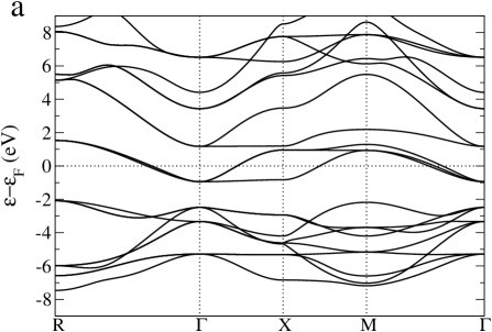
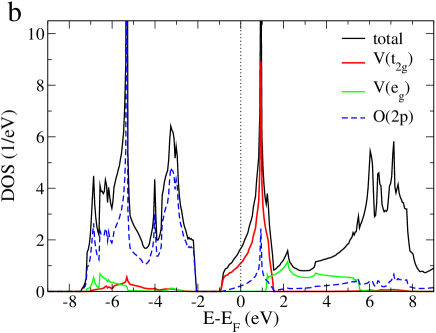
Figure 2: (Color online) (a) LDA data for SrVO₃ calculated with the MBPP code. (a) Band structure. (b) DOS. For the local V$(3d)$/O$(2p)$-DOS the cutoff radius was half the nearest-neighbor distance, respectively.

Figure 2 shows the band structure and the DOS within LDA. The data reveals that there is an isolated group of partially occupied bands at the Fermi level, with a total bandwidth of 2.5 eV. For an ion at site $\mathbf{R}$ the local orbital density matrix $n^{(l)}_{mm^{\prime}}$$\sim$$\sum_{\mathbf{k}\nu}f_{\mathbf{k}\nu}\langle\psi_{\mathbf{k}\nu}|K^{(l)}_{m}\rangle\langle K^{(l)}_{m^{\prime}}|\psi_{\mathbf{k}\nu}\rangle$ is a measure for the occupation probabilities within the set of, say cubic, harmonics $\{K^{(l)}_{m}\}$. In the case of SrVO₃ this matrix is diagonal, and it is seen in Fig. 2b that from such a projection the bands at $\varepsilon_{\rm{F}}^{\hfill}$ may be described as stemming dominantly from V$(t_{2g})$ orbitals. Since the three $t_{2g}$ orbitals, i.e, $\{d_{xy},d_{xz},d_{yz}\}$ are degenerate, they have equal contribution to the bands. Due to the full cubic symmetry the distinct $t_{2g}$ orbitals are nearly exclusively restricted to perpendicular planes which explains the prominent 2D-like logarithmic-peak shape of the DOS. The V$(e_{g})$ states have major weight above the Fermi level, whereas the O$(2p)$ states dominantly form a block of bands below $\varepsilon_{\rm{F}}^{\hfill}$ . The energy gap between the O$(2p)$ and $t_{2g}$ block amounts to 1.1 eV. In spite of the “block” characterization, there is still significant hybridization between the most relevant orbitals, i.e., V$(3d)$ and O$(2p)$, over a broad energy range.

III.1.2 Wannier functions

The low-energy physics of SrVO₃ is mainly determined by the isolated set of three $t_{2g}$-like bands around the Fermi level. This suggests the construction of an effective three-band Wannier Hamiltonian as the relevant minimal low-energy model. In the following, we construct Wannier functions associated with this group of bands, and also pick these three Wannier functions as generating the correlated subset $\mathcal{C}$, so that $\mathcal{W}$=$\mathcal{C}$ in the notations of the previous section. This choice of course implies that the resulting Wannier functions, though centered on a vanadium site, have also significant weight on neighbouring oxygen sites. More localized functions can indeed be obtained by keeping more bands in the Wannier constructions (i.e. by enlarging the energy window) and thus keeping $\mathcal{W}$ larger than $\mathcal{C}$, as described at the end of this subsection. However, we choose here to explore this minimal construction as a basis for a DMFT treatment and show that it actually gives a reasonable description of this material.

Figure 3: (Color online) $t_{2g}$ bands for SrVO₃ using different schemes to compute the $t_{2g}$ Wannier functions (and the underlying LDA band structure or potential). dark: MLWF(MBPP), dashed-red (dashed-gray): MLWF(FLAPW) and green (light gray): NMTO(LMTO-ASA). The $t_{2g}$ bandwidth is marginally larger in FLAPW, leading to small differences.

Figure 3 exhibits the Wannier bands obtained within our three utilized schemes: maximally-localized WFs from the MBPP and FLAPW codes (abbreviated in the following respectively by MLWF(MBPP) and MLWF(FLAPW)) and the NMTO scheme used as a postprocessing tool on top of the LMTO-ASA code (denoted as NMTO(LMTO-ASA)). For the MLWF construction a starting guess for the WFs was provided by utilizing atomic-like functions with $t_{2g}$ symmetry centered on the V site. Some details on the construction of the NMTO-WFs are provided in Appendix C. Both MLWF and NMTO schemes yield bands identical to the LDA bands. The small discrepancies seen in Fig. 3 are due to differences in the self-consistent LDA potentials. This overall agreement between the different methods reflects the coherent LDA description for this material.

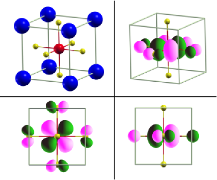
Figure 4: (Color online) $t_{2g}$-like MLWF $w_{xy}$ for SrVO₃ derived from the MBPP code. First row: SrVO₃ structure with Sr (large blue/dark), V (red/gray) and O (small yellow/light gray) and perspective view on $w_{xy}$. Second row: $w_{xy}$ viewed along the $c$ axis and along $a$ axis. The contour value $w_{xy}^{(0)}$ was chosen as 0.05 (a.u.)^-3/2.

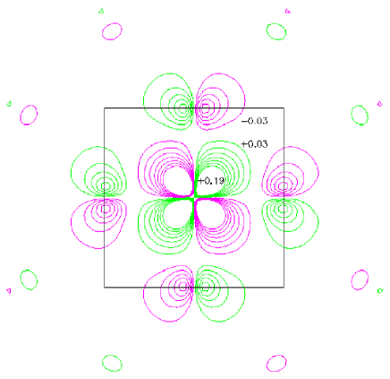
Figure 5: (Color online) Contour-lines plot of the $t_{2g}$-like MLWF $w_{xy}$ for SrVO₃. Distinct contour values (in (a.u.)^-3/2) are given in the plot.

Although all three sets of WFs span the same Hilbert space, and the bands are therefore the same, the MLWFs and the WFs obtained by symmetrically orthonormalizing the NMTO set are not necessarily identical. In order to compare the Wannier orbitals, we generated the set $\{w_{m}(\mathbf{r})\}$ within a (3$\times$3$\times$3) supercell on a (120$\times$120$\times$120) real-space mesh. As an example, Fig. 4 shows the $t_{2g}$-like $w_{xy}(\mathbf{r})$ Wannier orbital for a chosen constant value $w^{(0)}_{xy}$ as obtained from the MLWF(MBPP) construction. By symmetry, all three Wannier orbitals come out to be centered on the V site. A general contour plot for $w_{xy}(\mathbf{r})$ is given in Fig. 5. The Wannier orbitals show clear $t_{2g}$ symmetry, but in addition have substantial oxygen character, $\pi$-O($2p$) in particular. The important hybridization between the V($t_{2g}$) and O($2p$) atomic-like orbitals seen in Fig. 2 is explicitly transfered in the Wannier orbital. By comparing the three different sets of Wannier orbitals we find remarkably close agreement. Thus the MLWF and NMTO constructions provide nearly identical vanadium $t_{2g}$ Wannier orbitals in the case of cubic SrVO₃. A detailed comparison is shown in Fig. 6 where the WFs are plotted along specific directions.

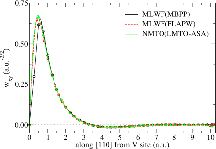
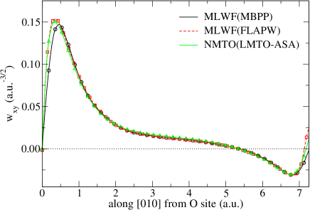
Figure 6: (Color online) (a) $t_{2g}$-like $w_{xy}$ WF. (a) From V to V along [110], and (b) from O to O along [010].

Table 1: Spread $\langle r^{2}\rangle$ of the V-centered $t_{2g}$ WFs for SrVO₃. We employed a (8$\times$8$\times$8) $k$-point mesh for the construction of the MLWFs. The spreads were calculated in two ways. First from the $k$-space integration performed in in the MLWF code, and second via an $r$-space integration within a (3$\times$3$\times$3) supercell. Additionally shown is the respective normalization of the WFs within this supercell. Finally, for completeness the $\Omega$ value minimized within the MLWF construction is also given, even if due to the complete degeneracy it reduces to three times the spread $\langle r^{2}\rangle$.

scheme	$\langle r^{2}\rangle$ (a.u.2)	norm	$\Omega$ (a.u.2)
	$\mathbf{k}$ space     $\mathbf{r}$ space	$\mathbf{r}$ space	$\mathbf{k}$ space
MLWF(MBPP)	6.86         6.64	0.998	20.57
MLWF(FLAPW)	6.96         6.75	0.997	20.93
NMTO(LMTO-ASA)	-             6.82	0.995	-
Ref. [Solovyev, 2006]	8.46	-	-

From these graphs it may be seen that the MLWF(MBPP) slightly disagrees with the WFs from the two other schemes close to the nuclei. This discrepancy is due to the pseudization of the crystal wave functions close to the nucleus. Although the $3d$ wave function is nodeless, the pseudo wave function is modified in order to provide an optimized normconserving pseudopotential. However, this difference in the WFs has no observable effect on the description of the bonding properties as outlined in general pseudopotential theory Harrison (1960); Heine (1970) (see also Tab. 2). Only marginal differences between the different WFs can be observed away from the nuclei. Generally, the fast decay of the WFs is documented in Fig. 6. In this respect, Table 1 exhibits the values for the spread $\langle r^{2}\rangle$ of the WFs from the different schemes. The MBPP and FLAPW implementations of the MLWFs have spreads which differ by 2$\%$. Since for the MLWFs the spread has been minimized, that of the NMTO-WFs should be larger, and it indeed is, but merely by a few per cent. So in this case the NMTO-WFs may be seen as maximally localized, also in the sense of Ref. [Marzari and Vanderbilt, 1997]. A substantially larger value for the spread is however obtained from the orthonormal LMTOs, as seen from Ref. [Solovyev, 2006].

To finally conclude this part of the comparison, we deduced the relevant near-neighbor hopping integrals from the real-space Hamiltonian in the respective Wannier basis, given in Table. 2. The dominance of the nearest-neighbor hopping in connection with the fast decay of the remaining hoppings clearly demonstrates the strong short-range bonding in SrVO₃. The close agreement of the hoppings between the three different Wannier schemes again underlines their coherent description of this material. It can be concluded that although conceptually rather different, MLWF and NMTO provide a nearly identical minimal Wannier description for SrVO₃. The small numerical differences seem to stem mainly from the differences in the electronic-structure description within the distinct band-structure methods.

Table 2: Symmetry-inequivalent intersite hopping integrals $H_{yz,yz}$ for SrVO₃. Energies are in meV.

$xyz$	001	100	011	101	111	002	200
MLWF(MBPP)	-260.5	-28.2	-83.1	6.5	-6.0	8.4	0.1
MLWF(FLAPW)	-266.8	-29.2	-87.6	6.4	-6.1	8.3	0.1
NMTO(LMTO-ASA)	-264.6	-27.2	-84.4	7.3	-7.6	12.9	3.5

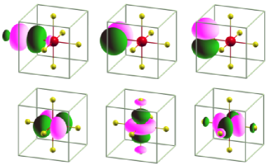
Figure 7: (Color online) Distinct WFs for SrVO₃ obtained from the MLWF construction using the MBPP code. First row: O($p_{x}$), O($p_{y}$) and O($p_{z}$) for a chosen oxygen site. Second row: V($t_{2g},xy$) as well as V($e_{g}$,$3z^{2}$-$r^{2}$) and V($e_{g}$,$x^{2}$-$y^{2}$). The contour value for each of the MLWFs was chosen as 0.05 (a.u.)^-3/2.

At the end of this subsection we want to draw attention to the fact that the performed minimal Wannier construction solely for the $t_{2g}$ bands is of course not the only one possible, as already mentioned above. Depicted in Fig. 7 are the WFs obtained by downfolding the LDA electronic structure of SrVO₃ to V($3d$) and O($2p$) states. Hence this corresponds to describing SrVO₃ via an 14-band model, i.e., three $p$ orbitals for three O ions and five $d$ orbitals for the single V ion in the unit cell. Due to minor degeneracies with higher lying bands (see Fig. 2) the disentangling procedure for the MLWF construction has to be used, but no relevant impact is detected in this case. Now there are distinct WFs for O($2p$) and V($3d$) with significantly smaller spreads. Individually the latter are in a.u.²: 2.61 for V($t_{2g}$) and 2.32 for V($e_{g}$), and 2.68 for $\sigma$-O($2p$) and 3.39 for $\pi$-O($2p$), resulting in a total spread of $\Omega$=40.75 a.u.².

III.1.3 LDA+DMFT calculations

Thanks to the simplicity of the perfectly cubic perovskite structure and the resulting degeneracy of the three $t_{2g}$ orbitals, SrVO₃ is a simple testing ground for first-principles dynamical mean-field techniques. In fact SrVO₃ is quite a unique case in which the calculation of the local Green’s function (22), which usually involves a $\mathbf{k}$ summation, can be reduced to the simpler calculation of a Hilbert transform of the LDA DOS. Indeed, because of the perfect cubic symmetry, all local quantities in the $t_{2g}$ subspace are proportional to the unit matrix: $G_{mm^{\prime}}^{\rm{loc}}(i\omega_{n})=G_{\rm{loc}}(i\omega_{n})\delta_{mm^{\prime}}$, $\Delta\Sigma_{mm^{\prime}}(i\omega_{n})=\Delta\Sigma(i\omega_{n})\delta_{mm^{\prime}}$ (as well as the LDA DOS $D_{mm^{\prime}}(\varepsilon)=D(\varepsilon)\delta_{mm^{\prime}}$ projected onto the orbitals $\chi_{m}$), so that (22) reduces to: $G_{\rm{loc}}(i\omega_{n})$=$\int\frac{d\varepsilon D(\varepsilon)}{i\omega_{n}+\mu-\varepsilon-\Delta\Sigma}$. Note however that this does not hold in general for other materials, as soon as the local quantities are no longer proportional to the unit matrix. Although many actual LDA+DMFT calculations in literature use this representation as an approximation to the correct form given by Eq. (22). In the calculations documented in this work we always used the more generic Hamiltonian representation and $\mathbf{k}$ summations.

Taking into account the strong correlations within the $t_{2g}$ manifold results in substantial changes of the local spectral function compared to the LDA DOS, namely a narrowing of the QP bands close to the Fermi level while the remaining spectral weight is shifted to Hubbard bands at higher energies. This general physical picture of the correlated metal can be understood already in the framework of the multi-orbital Hubbard model as the coexistence of QP bands with atomic-like excitations at higher energy. It directly carries through to the realistic case of SrVO₃ as studied in several previous works Liebsch (2003); Sekiyama et al. (2004); Pavarini et al. (2004); Nekrasov et al. (2005).

Moreover, an important feature of LDA+DMFT that emerges in the present case of a completely orbitally degenerate self-energy has been put to test against experiments. Indeed, in this special case Fermi-liquid behavior in conjunction with a $\mathbf{k}$-independent self-energy leads to the value of the local spectral function $\rho(\varepsilon)$ at the Fermi level being equal to its non-interacting counterpart just in the same way as in the one-band Hubbard model Müller-Hartmann (1989).

In this work we performed LDA+DMFT calculations for SrVO₃ by using the self-consistent LDA Wannier Hamiltonian $\mathbf{H}_{\rm{KS}}$ derived from the different band-structure codes, i.e., MBPP, LMTO-ASA and FLAPW, described above. As expected from the good agreement of the band structure and the Hamiltonians the resulting Green’s functions are identical within the statistical errors bars (see the inset of Fig. 8). Fig. 8 also displays the local spectral functions based on the MLWF(MBPP) scheme and calculated for different values of $U$. The “pinning” of $\rho(0)$, independently of the value of the interactions is clearly visible, despite the finite temperature of the calculations. This indicates that the calculations have indeed been performed at a temperature smaller than the QP (Fermi-liquid) coherence scale of this material.

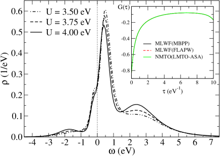
Figure 8: (Color online) Spectral function for SrVO3 for different values of $U$ resulting from LDA+DMFT in the MBPP implementation. Inset: comparison of Green’s functions from MBPP, FLAPW and NMTO implementations of LDA+DMFT for $U$=4 eV. In all calculations $J$=0.65 eV was used.

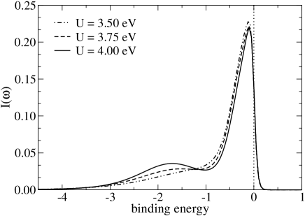
Figure 9: SrVO₃ spectral function convoluted with a Gaussian experimental resolution (assumed to be 0.15 eV) and with the Fermi function at $\beta$=30 eV^-1.

Figure 9 displays the local spectral function convoluted with an assumed experimental resolution of 0.15 eV and multiplied by the Fermi function. This quantity represents thus a direct comparison to angle-integrated photoemission spectra (albeit neglecting matrix elements, which can in certain circumstances appreciably depend e.g. on the polarization of the photons, see Ref. [Maiti et al., 2005]).

The general agreement with recent experimental data Sekiyama et al. (2004); Yoshida et al. (2005); Maiti et al. (2005); Wadati et al. (2006); Eguchi et al. (2006) is reasonable. Photoemission experiments locate the lower and upper Hubbard bands at energies about -2 eV to -1.5 eV Sekiyama et al. (2004); Maiti et al. (2005) and 2.5 eV Morikawa et al. (1995) respectively. In our calculations the lower Hubbard band extends between -2 eV to -1.5 eV, while the maximum of the upper Hubbard band is located at about 2.5 eV, for values of the Coulomb interaction $U$ of about 4 eV. However, we also confirm the findings of Ref. [Maiti et al., 2005] who point out that LDA+DMFT calculations generally locate the lower Hubbard band at slightly higher (in absolute value) binding energies than -1.5 eV, the energy where their data exhibits its maximum.

Concerning the choice of the Coulomb interaction $U$ different points of view can be adopted. First, one can of course choose to try to calculate $U$ itself from first principles by e.g. constrained LDA Dederichs et al. (1984); McMahan et al. (1988); Gunnarsson et al. (1989); Anisimov and Gunnarsson (1991); Cococcioni and de Gironcoli (2005) or RPA-based techniques Aryasetiawan et al. (2004); Solovyev and Imada (2005). Another option is to use it as an adjustable parameter and to determine it thus indirectly from experiments. While in the present case the order of magnitude of the interaction ($U$$\sim$3.5-5.5 eV) Sekiyama et al. (2004); Solovyev (2006); Aryasetiawan et al. (2006) is indeed known from first-principles approaches, the exact values determined from different methods still present a too large spread to be satisfactory for precise quantitative predictions. We therefore adopt the second point of view here, noting that $U$ values of around 4 eV reproduce well the experimentally observed Yoshida et al. (2005); Wadati et al. (2006); Inoue et al. (1998) mass enhancement of $\sim$1.8 to 2. The agreement concerning the position of the Hubbard bands seems to be fair, given the theoretical uncertainty linked to the analytical continuation procedure by maximum-entropy techniques and the spread in available experimental data. Still, it is conceivable that the determination of the precise position of the Hubbard bands could require more sophisticated methods than LDA+DMFT done with a static $U$ parameter, and that in fact we are facing the consequences of subtle screening effects which, within an effective three-band model, could only be described by a frequency-dependent interactionAryasetiawan et al. (2004).

III.2 $Cmc2_{1}$-BaVS₃

III.2.1 Structure and physical properties

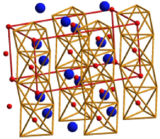
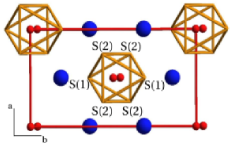
Figure 10: (Color online) BaVS₃ in the $Cmc2_{1}$ structure. The V ions are shown as smaller (red/gray) spheres, the Ba ions as larger (blue/dark) spheres.

The transition-metal sulfide BaVS₃ is also a $3d(t_{2g})^{1}$ system, but its physical properties are far more complex Booth et al. (1999); Whangbo et al. (2003) than those for the cubic perovskite SrVO₃ considered above. In a recent work Lechermann et al. (2005a, b), three of us have suggested that a correlation-induced redistribution of orbital populations is the key mechanism making the transition into a charge-density wave (CDW) insulating phase possible. Here, we use our Wannier formalism to make a much more refined study of this phenomenon and to calculate how correlations modify the Fermi-surface sheets of the metal. Also, this material is a challenging testing ground for the Wannier construction because of the strong hybridization between the transition-metal and ligand bands.

We first give a very brief summary of some of the physical properties of BaVS₃ of relevance to the present paper. At room temperature BaVS₃ exists in a hexagonal crystal structure (space group $P6_{3}/mmc$), with two formula units of BaVS₃ in the primitive cell. There are straight chains of face sharing VS₆ octahedra along the $c$ axis, and Ba ions in between. A continuous structural phase transition at $T_{\rm{S}}$$\sim$240 K reduces the crystal symmetry to orthorhombic, thereby stabilizing the $Cmc2_{1}$ structure, again with two formula units in the primitive cell. Now the VS₃ chains are zigzag-distorted in the $bc$ plane. In this phase, BaVS₃ is a quite bad metal, with unusual properties such as a Curie-Weiss susceptibility from which the presence of local moments can be inferred. At $\sim$70 K a second continuous phase transition takes place Graf et al. (1995); Mihály et al. (2000), namely a metal-insulator transition (MIT) below which BaVS₃ becomes a paramagnetic insulator. A doubling of the primitive unit cell Inami et al. (2002); Fagot et al. (2003, 2005) is accompanying the MIT. Together with large one-dimensional structural fluctuations along the chains Fagot et al. (2003) and additional precursive behavior for the Hall constant Booth et al. (1999) just above $T_{\rm{MIT}}$, the transition scenario is reminescent of a Peierls transition into a charge-density wave (CDW) state. Finally a third second order transition appears to occur at $\sim$30 K. This so-called “X” transition is of magnetic kind and shall announce the onset of incommensurate antiferromagnetic order Nakamura et al. (2000) in the insulator.

Here we want to focus on the orthorhombic ($Cmc2_{1}$) structure (see Fig. 10) at $T$=100 K, i.e., just above the MIT. Ten ions are incorporated in the primitive cell. Whereas the two Ba and two V ions occupy (4a) sites, there are two types of sulfur ions. Two S(1) ions are positioned at (4a) apical sites on the $b$ axis, while four S(2) ions occupy (8b) sites. The lattice parameters are: Ghedira et al. (1986) $a$=12.7693 a.u., $b$=21.7065 a.u. and $c$=10.5813 a.u..

III.2.2 Band structure

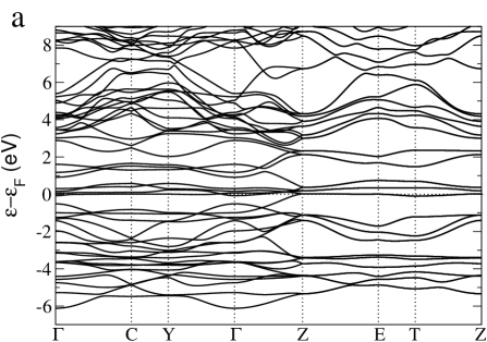
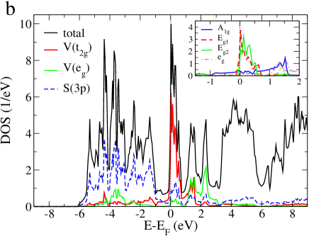
Figure 11: (Color online) LDA data for BaVS₃ after the MBPP method. (a) band structure and(b) DOS. For the local V$(3d)$/S$(3p)$-DOS the cutoff radius was half the minimum nearest-neighbor distance, respectively. The inset in (b) shows the symmetry-adapted local V$(3d)$-DOS close to the Fermi level.

Figure 11 depicts the LDA band structure and DOS of $Cmc2_{1}$-BaVS₃. To allow for orbital resolution, the local DOS was again projected onto symmetry-adapted cubic harmonics by diagonalizing $n^{(d)}_{mm^{\prime}}$. It is seen that the bands at $\varepsilon_{\rm{F}}^{\hfill}$ have dominant $t_{2g}$ character, however they still carry sizeable S($3p$) weight. Furthermore, the $t_{2g}$-like bands are now not isolated but strongly entangled with S($3p$)-like bands. Due to the reduction of symmetry from hexagonal to orthorhombic, the $t_{2g}$ manifold splits into $A_{1g}$ and $E_{g}$ . The two distinct $E_{g}$ states will be denoted in the following $E_{g1}$ and $E_{g2}$. Being directed along the $c$ axis, the $A_{1g}$ orbital points towards neigboring V ions within a chain and the corresponding band (see Fig. 12a) shows a folded structure because of the existence of two symmetry-equivalent V ions in the unit cell. The folded $A_{1g}$ band has a bandwith of 2.7 eV, while $E_{g}$ states form very narrow (0.66 eV) bands right at the Fermi level.

From the LDA DOS it seems that a projection onto $t_{2g}$-like orbitals close to the Fermi level by diagonalizing $n^{(d)}_{mm^{\prime}}$ is, at least to a first approximation, meaningfulLechermann et al. (2005a). However there is a substantial S($3p$) contribution close to $\varepsilon_{\rm{F}}^{\hfill}$ and generally large charge contributions in the interstitial. Hence establishing a very accurate correspondance between relevant bands and orbitals is not possible in such a way. In contrast, the Wannier schemes discussed above are quite suitable for dealing with this situation. To be specific, we applied the MLWF scheme in the new MBPP implementation to this problem.

Besides providing a test for the MLWF scheme, the present study will allow us to make considerably more precise the findings of Ref. [Lechermann et al., 2005a] regarding the crucial role of correlation-induced changes in the orbital populations, and most notably to clarify how these changes can modify the Fermi surface (FS) of this material in such a way that favorable conditions for a CDW transition indeed hold. Key to the physics of BaVS₃ is the simultaneous presence of two quite distinct low-energy states, the rather delocalized $A_{1g}$ and quite localized $E_{g}$ , among which the electronic density with one electron per vanadium has to divide itself. Depending on temperature, the associated orbital populations correspond to the best compromise between gain of kinetic energy and cost of potential energy. As it appears, this compromise seems to be realized by a CDW state below the MIT. However, as revealed in several electronic structure studies Mattheiss (1995); Whangbo et al. (2003); Lechermann et al. (2005a), a DFT-LDA description of BaVS₃ does not explain the occurence of a CDW instability. Though the mainly $A_{1g}$-like band appears to be a promising candidate, a nesting scenario in agreement with the critical wave vector ${\mathbf{q}}_{c}$=$0.5{\bf c}^{*}$ from experiment Fagot et al. (2003) is not realizable. In Fig. 12a we elaborated a so-called “fatband” Jepsen and Andersen (1995) resolution of the LDA band structure close to the Fermi level, which is helpful to reveal the respective band character to a good approximation. Thereby the Bloch function associated with a given $k$-point and eigenvalue is projected onto orthonormal symmetry-adapted local orbitals (determined as usual by diagonalizing the local orbital density matrix $n^{(l)}_{mm^{\prime}}$). The resulting magnitude of the overlap is depicted as a broadening of the corresponding band. Here it is seen that $A_{1g}$-like band cuts the Fermi level close to the boundary of the BZ along $\Gamma$-Z, i.e., along the $c^{*}$ axis in reciprocal space. Since the Z point is located at $k_{z}$=$0.5c^{*}$, in numbers this amounts to 2$k_{F}$=0.94 for the $A_{1g}$-like band within LDA, nearly twice the experimental value determined for the nesting vector. Furthermore, also other parts of the LDA FS are out of reach for ${\mathbf{q}}_{c}$, as the $A_{1g}$ sheet is too extended and additionally strongly warped (see also Fig. 19b). In other words, LDA apparently overestimates the population of the more itinerant $A_{1g}$ state.

Moreover the role of the electrons with strong $E_{g}$ character at the MIT is not obvious. When approaching $T_{\rm{MIT}}$ these nearly localized electrons should surely contribute to the Curie-Weiss form of the magnetic susceptibility Mihály et al. (2000); Lechermann et al. (2005a). In fact the “bad-metal” regime Graf et al. (1995) above the MIT, including significant changes in the Hall coefficient Booth et al. (1999), might largely originate from scattering processes involving the $E_{g}$ electrons. But even if the $A_{1g}$ bands become gapped at the MIT, from an effective single-particle LDA viewpoint the remaining $E_{g}$ bands may still ensure the metallicity of the system. We therefore believe for several reasons that correlation effects beyond LDA are important Lechermann et al. (2005a) for an understanding of the physics of BaVS₃. We will further outline relevant mechanisms, now based on a more elaborate Wannier scheme, in section III.2.4.

III.2.3 Wannier functions

Figure 12: (Color online) (a) $t_{2g}$ fatband resolved band structure of BaVS₃. The color code is as follows: $A_{1g}$ (blue/dark), $E_{g1}$ (red/gray) and $E_{g2}$ (green/light gray). (b) downfolded $t_{2g}$ Wannier bands (light blue/light gray) for BaVS₃ obtained from the MLWF construction using the MBPP code.

The central difficulty in constructing $t_{2g}$-like WFs for BaVS₃ is the strong hybridization between V($3d$) and S($3p$), leading to a substantial entanglement between the two band manifolds. In detail, whereas the two $E_{g}$ states form four very narrow bands, mainly confined to the Fermi level, the folded $A_{1g}$ band extends into the dominantly S($3p$)/V($e_{g}$) band manifolds lower/higher in energy. This entanglement is documented in Fig. 12a by significant “jumps” of the corresponding $A_{1g}$ fatband between different bands. One may of course downfold the BaVS₃ band structure including not only V($t_{2g}$) but also S($3p$) and V($e_{g}$) orbitals. However, in this work we wanted to investigate the properties and reliability of the minimal, i.e., $t_{2g}$-only, model. In the following we discuss the results obtained via the MLWF construction. Corresponding studies were also performed with an NMTO basis set leading to the same physical picture. But a detailed comparison would at this point shift the attention from the investigated physical mechanisms.

Table 3: Wannier centers $\mathbf{R}_{w}$ and spread $\langle r^{2}\rangle$ of $t_{2g}$-like MLWFs for BaVS₃ constructed from a (6$\times$6$\times$6) $k$-point mesh. The positions of the symmetrically equivalent V sites in cartesian coordinates read $\mathbf{R}_{\rm{V(1)}}$=(0.00,0.46,-0.01) a.u. and $\mathbf{R}_{\rm{V(2)}}$=(0.00,-0.46,5.28) a.u.. The V(2) site is symmetry-related to the V(1) site by the symmetry operation $C_{2}^{(z)}\mathbf{R}_{\rm{V(1)}}$+0.5.

WF	$\mathbf{R}_{w}$ (a.u.)	$\mathbf{R}_{w}-\mathbf{R}_{\rm{V}}$ (a.u.)	$\langle r^{2}\rangle$ (a.u.2)
$A_{1g}$, V(1)	0.00, 0.75, -0.20	0.00, 0.30, -0.19	16.57
$E_{g1}$, V(1)	0.00, 0.64,  0.38	0.00, 0.18,  0.39	17.55
$E_{g2}$, V(1)	0.00, 1.02, -0.32	0.00, 0.56, -0.31	17.53

Table 4: Wannier centers $\mathbf{R}_{w}$ and spread $\langle r^{2}\rangle$ as in Tab. 4, now in the crystal-field basis.

WF	$\mathbf{R}_{w}$ (a.u.)	$\mathbf{R}_{w}-\mathbf{R}_{\rm{V}}$ (a.u.)	$\langle r^{2}\rangle$ (a.u.2)
$A_{1g}$, V(1)	0.00, 0.75, -0.17	0.00, 0.30, -0.16	16.60
$E_{g1}$, V(1)	0.00, 0.65,  0.34	0.00, 0.19,  0.35	17.55
$E_{g2}$, V(1)	0.00, 1.02, -0.32	0.00, 0.56, -0.31	17.53

In order to downfold onto $\{A_{1g},E_{g1},E_{g2}\}$ we employed the disentangling procedure Souza et al. (2001) of the MLWF construction. The WFs were initialized via cubic harmonics adapted to an ideal local hexagonal symmetry. To the aim of correct disentangling of the six Wannier target bands we provided twenty bands in an outer energy window around the Fermi level for the construction of $M_{\nu\nu^{\prime}}^{(\mathbf{k},\mathbf{q})}$. In order to reproduce the LDA FS and the band dispersions close to the Fermi level correctly, we additionally forced the Wannier bands in an inner energy window near $\varepsilon_{\rm{F}}^{\hfill}$ to coincide with the true LDA bands Souza et al. (2001). The initial WFs correspond to an optimized $\Omega_{I}$=101.58 a.u.² and a starting value $\tilde{\Omega}$=3.62 a.u.², hence a total $\Omega$ of 105.19 a.u.² for the chosen energy windows. After $\sim$50000 iteration steps $\Omega$ finally converged to 103.30 a.u.². During the minimization process, adaptation of the WFs to the true orthorhombic symmetry was clearly observed by the occurence of distinct steps in $\Omega$. The resulting $t_{2g}$ Wannier bands are shown in Fig. 12b in comparison with the original LDA band structure. It is seen that the Wannier bands at the Fermi level are truly pinned to the original LDA bands. Furthermore the interpolated lowest/highest Wannier band follows nicely the former $A_{1g}$ fatbands. The same $t_{2g}$ dispersion is also obtained within an NMTO contruction.

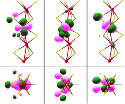
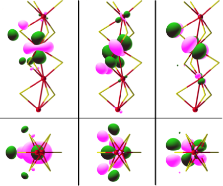
Figure 13: (Color online) $t_{2g}$ Wannier orbitals for BaVS₃ forming the maximally-localized basis. The columns from left to right show the $A_{1g}$, $E_{g1}$ and $E_{g2}$ orbitals, while the second row displays the orbitals viewed along the $c$ axis. There the $a$ axis is vertically oriented, while the $b$ axis horizontally. The contour value for each of the orbitals was chosen as 0.045 (a.u.)^-3/2.

Figure 14: (Color online) $t_{2g}$ Wannier orbitals for BaVS₃ forming the crystal-field basis. The order of the columns and row same as in Fig.14. Note that the $E_{g2}$ orbital remains invariant under this transformation. The contour value for each of the orbitals was equally chosen as 0.045 (a.u.)^-3/2.

Table 5: Hopping integrals between the $t_{2g}$ Wannier orbitals of BaVS₃ in the maximally-localized basis. The term ’00$\frac{1}{2}$’ shall denote the hopping to the nearest-neighbor V site within the unit cell. One of the nearest-neighbor V ions in the $ab$ plane is located at ’100’, while ’110’ and ’$\bar{1}$10’ are closest V ions along $a$ and $b$, respectively. Energies in meV.

	$A_{1g}$-$A_{1g}$	$E_{g1}$-$E_{g1}$	$E_{g2}$-$E_{g2}$	$A_{1g}$-$E_{g1}$	$A_{1g}$-$E_{g2}$	$E_{g1}$-$E_{g2}$
000	414.4	218.0	235.6	40.8	0.0	0.0
00$\frac{1}{2}$	-441.5	-24.7	-12.4	-242.6	0.0	0.0
001	-66.0	-5.4	2.7	-8.9	0.0	0.0
100	-30.4	8.5	-26.1	-15.8	16.4	-10.9
110	-17.4	-84.4	29.2	-16.5	-0.7	11.6
$\bar{1}$10	1.6	1.7	-5.5	-1.8	0.0	0.0

Table 6: Hopping integrals as in Tab. 6 but now in the crystal-field basis.

	$A_{1g}$-$A_{1g}$	$E_{g1}$-$E_{g1}$	$E_{g2}$-$E_{g2}$	$A_{1g}$-$E_{g1}$	$A_{1g}$-$E_{g2}$	$E_{g1}$-$E_{g2}$
000	422.6	209.8	235.6	0.0	0.0	0.0
00$\frac{1}{2}$	-510.5	44.3	-12.4	-145.7	0.0	0.0
001	-85.5	14.2	2.7	7.1	0.0	0.0
100	-35.4	13.6	-26.1	-7.0	-14.0	13.9
110	-26.3	-75.5	29.2	-28.1	-1.6	-11.5
$\bar{1}$10	1.2	2.1	-5.5	-1.7	0.0	0.0

Table 4 reveals that the Wannier spreads are significantly larger than for the $t_{2g}$ WFs in SrVO₃. The spread for the $A_{1g}$ WF is slightly smaller than those for the $E_{g}$ orbitals. Moreover, it is seen from Tab. 4 that the Wannier centers are shifted from the V sites. This may be explained by the low symmetry of the $Cmc2_{1}$-BaVS₃ structure, since already from the missing inversion symmetry in the site symmetry for the V ion there is no need for the WFs to be centered on the V sites Marzari and Vanderbilt (1997). Additionally, the explicit inclusion of the sulfur contribution to the $t_{2g}$ WFs leads to directed Wannier orbitals. The latter may be inspected in Fig. 14, where we plotted the three Wannier orbitals associated with the first V ion in the unit cell (the other three are directly related by symmetry due to the equivalence of the V ions). Indeed the $A_{1g}$-like orbital is directed along the $c$ axis, whereby the zigzag distortion of the chains causes some tilting. Note that the orbitals have some weight on neighboring V sites. As especially observable for the $E_{g1}$-like orbital, this weight has local $e_{g}$ symmetry. Thus the MLWF construction reproduces here the intuitively formulated symmetry constraints imposed in the NMTO construction Andersen and Saha-Dasgupta (2000); Andersen et al. (2000); Zurek et al. (2005). This symmetry relation between WFs on neigboring sites has also been noted for the V₂O₃ compound Saha-Dasgupta et al. (to be published), half-metallic ferromagnets Yamasaki et al. (2006b) and, most dramatically, for Na_xCoO₂ compounds Andersen et al. (to be published). The $E_{g1}$ orbital is mainly oriented in the plane defined by the S(2) ions, while $E_{g2}$ remains in the corresponding perpendicular plane. Accordingly, $E_{g1}$ has stronger weight on the S(2) ions, whereas $E_{g2}$ connects to the apical S(1). For $A_{1g}$ the sulfur distribution is in-between, yet favoring the nearest-neighbor S(1).

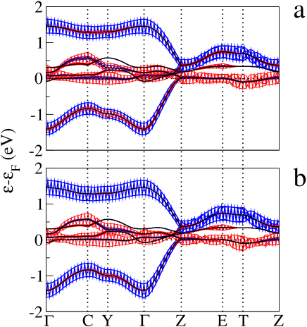
Figure 15: (Color online) $t_{2g}$ Wannier fatbands for BaVS₃, (a) with respect to the maximally-localized basis, and (b) with respect to the crystal-field basis (see text). Color coding: $A_{1g}$-like WF (blue/dark), $E_{g1}$-like WF (red/gray).

In order to investigate the properties of these WFs in more detail, Tab. 6 displays the hopping integrals for relevant paths on the lattice. One immediately realizes that while the $E_{g2}$ orbital remains isolated, there is a sizable hybridization between the $A_{1g}$ and $E_{g1}$ Wannier orbitals. The latter hybridization clearly couples $A_{1g}$ and $E_{g1}$ in view of the zigzag distortion along the $b$ axis (see Fig. 14) This coupling should play an important role for the understanding of the whole BaVS₃ phase diagram, also crucial for the hexagonal-to-orthorhombic structural transition Lechermann (to be published). Note also the dominant $E_{g1}$-$E_{g1}$ hopping along the $a$ axis, i.e. [110], which is in accordance with orbital extension of the corresponding WFs (see Fig. 14).

In Figure 15a we plot the disentangled (effective) $t_{2g}$ bands with a fatband resolution to reveal the respective contribution of the obtained MLWFs (for simplicity we do not plot the $E_{g2}$ fatband). One can see that the $A_{1g}$ band carries substantial $E_{g1}$ weight (and vice versa) due to their sizeable hybridization in the maximally-localized basis. This is is somehow counter-intuitive to the original low-energy picture of a broader $A_{1g}$ band and narrower $E_{g1}$ band. Though some minor $A_{1g}$-$E_{g1}$ hybridization in the $\Gamma$-C-Y plane is in line with the original LDA fatbands, it seems that this hybridization is slightly over-represented in the maximally-localized basis. Surely, the latter basis is not a priori physically designated, and it might be that the the straightforward MLWF construction does not provide the most suitable physical Wannier basis for the description of BaVS₃.

With the aim of reducing this strong $A_{1g}$-$E_{g1}$ hybridization in the maximally-localized basis, we diagonalized the on-site Wannier Hamiltonian $\mathbf{H}_{\rm{KS}}^{(\mathbf{T}=\mathbf{0})}$=$\sum_{\mathbf{k}}\mathbf{H}_{\rm{KS}}(\mathbf{k})$ and transformed $\mathbf{H}_{\rm{KS}}(\mathbf{k})$ into the so-called crystal-field basis (e.g. also utilized in Ref. [Pavarini et al., 2005]). The (again unitary) transformation is explicitly written as:

$$\begin{pmatrix}w^{\rm{(cf)}}_{A_{1g}}\\ w^{\rm{(cf)}}_{E_{g1}}\\ w^{\rm{(cf)}}_{E_{g2}}\end{pmatrix}=\begin{pmatrix}0.981&0.196&0.000\\ -0.196&0.981&0.000\\ 0.000&0.000&1.000\\ \end{pmatrix}\begin{pmatrix}w^{\rm{(ml)}}_{A_{1g}}\\ w^{\rm{(ml)}}_{E_{g1}}\\ w^{\rm{(ml)}}_{E_{g2}}\end{pmatrix}\,,$$

where the superscript ’cf’ marks the crystal-field basis and ’ml’ the maximally-localized basis. This procedure obviously decouples $A_{1g}$ and $E_{g1}$ on average and provides a true adaption to the local symmetry at the V site. Within this new basis the $A_{1g}$ hopping along the $c$ axis is strenghtend at the cost of a reduced $A_{1g}$-$E_{g1}$ hybridization (see Tab. 6). In addition, the sign of the near-neighbor $E_{g1}$-$E_{g1}$ hopping is changed from negative to positive. The Wannier fatbands promote now more the elucidated picture of the $E_{g1}$ bands being confined to $\varepsilon_{\rm{F}}^{\hfill}$ (see Fig. 15b). Only minor changes may be observed however in the same contour plot for the transformed Wannier orbitals, as seen in Fig. 14. The $A_{1g}$ Wannier orbital is now more reminescent of a $d_{3z^{2}-r^{2}}$ orbital perpendicular to $c$ and $E_{g1}$ is slightly tilted out of the plane defined by the S(2) ions. Correspondingly, the numbers for the Wannier centers and spreads have changed only marginally, as seen in Tab. 4.

By summing the spreads one easily checks that $\Omega$ is now marginally larger than in the original maximally-localized basis, which is of course consistent with the fact that the original set was constructed by minimizing the spread.

Although the real-space quantities truly do not differ much, the electronic structure representation is very sensitive to rather minor changes in the basis. This is not only seen for the hoppings (cf. Tabs 6,6) but may also be observed when comparing the different orbitally-resolved DOS originating from the two Wannier basis sets (see Fig. 16). There, in general the overall lowdimensional character of the $A_{1g}$ band is emphasized within the minimal Wannier set. Note the reduced DOS magnitude close to the Fermi energy for the latter band in the crystal-field basis. On the other hand the $A_{1g}$ DOS is reinforced below the Fermi energy at the cost of a reduced $E_{g1}$ DOS. This effect precisely reflects the low-energy confinement of $E_{g1}$ in the crystal-field basis.

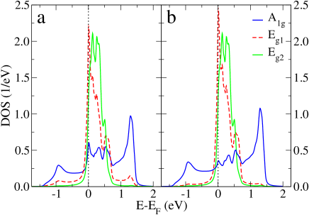
Figure 16: (Color online) $t_{2g}$ Wannier DOS for BaVS₃. (a) In the maximally-localized basis, and (b) in the crystal-field basis.

III.2.4 LDA+DMFT calculations

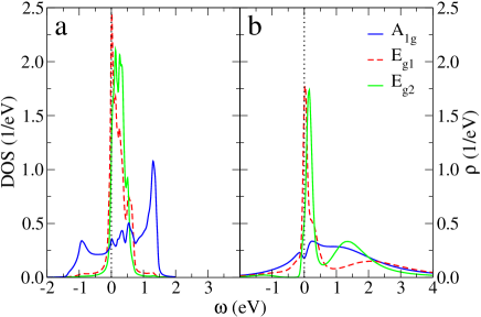
Figure 17: (Color online) (a) Wannier DOS for BaVS₃ in the crystal-field basis. (b) corresponding $\mathbf{k}$-integrated spectral function for BaVS₃ within LDA+DMFT for $\beta$=30 eV^-1.

It was pointed out in Ref. [Lechermann et al., 2005a] that correlation effects are important for an understanding of the MIT in BaVS₃. From LDA+DMFT calculations using as an input the symmetry-adapted local DOS for $\{A_{1g},E_{g1},E_{g2}\}$, a substantial charge transfer from $A_{1g}$ to $E_{g}$ was revealed. The latter was associated with a reduced Fermi wave vector $k_{F}$ for the $A_{1g}$ band, allowing for the possibility of the observed CDW instability. In this section we will check, and also considerably refine these earlier results. Indeed, because the Wannier construction allows us to study this intricate material within a Hamiltonian formalism which allows us to address $\mathbf{k}$-resolved issues, we are now in a position to study in detail the correlation-induced changes of the Fermi surface of BaVS₃. Since we believe that the crystal-field basis constructed in the last section is more closely adapted to the physics of BaVS₃ than the direct MLWF basis, we will use this basis in the following. We made cross checks using the MLWF basis, and will comment on relevant differences.

For the new LDA+DMFT calculations we chose $U$=3.5 eV, $J$=0.7 eV. Although no concrete knowledge about the value of $U$ for BaVS₃ is known, we believe that the latter values are in agreement with realistic values for this compound Lechermann et al. (2005a). The single-site impurity problem was solved for $\beta$=30 eV^-1 ($\sim$390 K). A number of 128 time slices and up to 10⁶ Monte-Carlo sweeps were used in the actual calculations.

In Fig. 17 the orbital-resolved $\mathbf{k}$-integrated spectral function is shown in comparision to the corresponding LDA DOS in the Wannier basis. The band-narrowing effect is clearly visible. Additionally, the tendency towards the opening of a pseudo-like gap in the $A_{1g}$ band may be oberved. This latter feature is missing when using the maximally-localized Wannier basis.

Table 7: Band fillings for BaVS₃ from LDA+DMFT within the crystal-field Wannier basis.

$\beta$ (eV-1)	$U$,$J$ (eV)	$A_{1g}$	$E_{g1}$	$E_{g2}$
$\rightarrow\infty$	0.0, 0.0	0.59	0.31	0.10
30	0.0, 0.0	0.58	0.30	0.12
30	3.5, 0.7	0.41	0.45	0.14

Table 7 shows final occupations of the Wannier orbitals varying with temperature and interaction strength. The values for ($\beta\rightarrow\infty$,$U$=$J$=0) correspond to the LDA limit. Comparing with LDA values obtained in Ref. [Lechermann et al., 2005a], the current LDA orbital polarization is not so severe in the Wannier description. This is due to the fact that in Ref.[Lechermann et al., 2005a] we used an empirical downfolding for the local DOS, merging most sulfur character with the $A_{1g}$ band. Since in the Wannier description the downfolding of sulfur now also puts some weight on the $E_{g}$ states, their filling is somehow increased. Nonetheless, turning on $U$ does transfer sizable charge between the orbitals, hence the correlation effects envisioned in Ref. [Lechermann et al., 2005a] are indeed confirmed in the more elaborate Hamiltonian framework with WFs. However, due to the now resolved $A_{1g}$-$E_{g1}$ hybridization, the charge transfer dominantly takes place between these two orbitals, leaving $E_{g2}$ as a mere “spectator”. These interorbital charge transfers suggest that the FS of this material might actually be quite different than predicted by LDA, namely that the relative size of the various FS sheets may be significantly changed. A word of caution is in order however: the Luttinger theorem Luttinger (1960) only constrains the total $k$-space volume encompassed by all sheets of the FS, and stipulates that it should correspond to one electron per vanadium for the present material, independently of interactions, in the metallic phase. There is no a priori theoretical relation between the volume of each individual sheet and the orbital populations as calculated above. Nonetheless, the reduction of the $A_{1g}$ population in favor of $E_{1g}$ may provide a hint that there is a corresponding shrinking of the $A_{1g}$ FS sheet. We now address in details whether this shrinking does occur and along which directions in reciprocal space.

In order to investigate $\mathbf{k}$-resolved effects of correlations, one must in principle determine the real-frequency self-energy. Since we are however mainly interested in the Fermi surface of the interacting system, we can extract the low-energy expansion of $\Sigma(\omega)$ from our QMC calculation in the form:

$$\Re\Sigma_{mm^{\prime}}(\omega+i0^{+})\simeq\Re\Sigma_{mm^{\prime}}(0)+\left(1-[\mathbf{Z}^{-1}]_{mm^{\prime}}\right)\omega+\cdots,$$ (28)

where $\mathbf{Z}$ describes the matrix of QP weights. The QP dispersion relation is then obtained from the poles of the Green’s function:

$$\mbox{det}[\omega_{\mathbf{k}}\mathbf{\openone}-\mathbf{Z}\left(\mathbf{H}_{\rm{KS}}(\mathbf{k})+\Re\mathbf{\Sigma}(0)-\mu\mathbf{\openone}\right)]=0\quad.$$ (29)

Correspondingly, the FS in the interacting system is defined by

$$\mbox{det}[\mu\mathbf{\openone}-\mathbf{H}_{\rm{KS}}(\mathbf{k})-\Re\Sigma(0)]=0\quad.$$ (30)

From Eqs. (29-30) one understands that $\Re\mathbf{\Sigma}(0)$ provides an energy shift to the LDA bands. The direction and magnitude of this shift depends at each $k$-point on the amount of the contributing orbital character, since $\Re\mathbf{\Sigma}(0)$ is explicitly orbital-dependent. Hence although our self-energy is explicitly $\mathbf{k}$ independent within single-site DMFT, one may still evaluate some $\mathbf{k}$-dependent effects due to the explicit $\mathbf{H}_{\rm{KS}}(\mathbf{k})$ inclusion.

From the converged self-energy matrix $\mathbf{\Sigma}(i\omega_{n})$ we derived $\Re\mathbf{\Sigma}(0)$ and $\mathbf{Z}$ via Pade approximation. Table 8 displays the two matrices.

Table 8: $\Re\mathbf{\Sigma}(0)$ (in eV) and $\mathbf{Z}$ for BaVS₃ in the Wannier crystal-field basis from LDA+DMFT.

		$\Re\mathbf{\Sigma}(0)$			$\mathbf{Z}$
	$A_{1g}$	$E_{g1}$	$E_{g2}$	$A_{1g}$	$E_{g1}$	$E_{g2}$
$A_{1g}$	0.35	-0.01	0.00	0.57	-0.02	0.00
$E_{g1}$	-0.01	-0.03	0.00	-0.02	0.52	0.00
$E_{g2}$	0.00	0.00	0.03	0.00	0.00	0.58

First, the symmetry of these matrices follows the earlier observations, hence there is some $A_{1g}$-$E_{g1}$ coupling also reflected in the self-energy. The band renormalization cast into $\mathbf{Z}$ are roughly of the same order, with a slight maximum band narrowing close to a factor of two for the $E_{g1}$ band. Since we want to elucidate FS deformations due to correlations, looking for an explanation for the CDW instability, the $\Re\mathbf{\Sigma}(0)$ matrix is of high relevance. From that, states with strong $A_{1g}$ character should considerably shifted upwards in energy, while for dominantly $E_{g}$ states it depends on their symmetry. Bands with $E_{g1}$ character should be shifted down, whereas those with $E_{g2}$ character should be shifted up. The latter discrepancy may be relevant to understand the opening of the gap at the MIT within the $E_{g}$ states. Since the dispersion of the $A_{1g}$-like band is highly anisotropic, i.e. 1D-like, the rather strong shifting should result in a major FS deformation, invoking the possibility for an arising CDW instability.

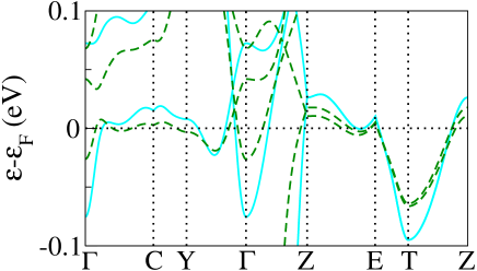
Figure 18: (Color online) $\mathbf{k}$-resolved correlation effect for BaVS₃. QP band structure from LDA+DMFT (darkgreen dashed/dark dashed) in comparision with the Wannier band structure based on LDA (cyan/light gray) close to the Fermi level.

Fig. 18 displays the QP band structure according to Eq. (29) close to the Fermi level. Using the linearized self-energy should be valid within the small energy window around $\varepsilon_{\rm{F}}^{\hfill}$ . Note first the overall narrowing of the bands since $Z$$<$1. The former statements concerning the respective shifts of the bands are accordingly reproduced. The electron pocket at the $\Gamma$ point was identified as $E_{g2}$ like (compare Fig. 12a) and hence is now shifted upwards. Roughly speaking, the system is getting rid of the $E_{g2}$ states when turning on correlations. Also the $E_{g1}$-like bands are considerably shifted downwards. In fact it is revealed in studies of the monoclinic phase below $T_{\rm{MIT}}$, that the internal $E_{g}$ splitting seems indeed realized in the way outlined above Lechermann (to be published). Moreover, the off-diagonal $A_{1g}$-$E_{g1}$ self-energy terms within LDA+DMFT lift the band degeneracy in the E-T-Z plane of the BZ. Originally it was argued Mattheiss (1995) within the LDA picture that the presence of the doubly-degenerated bands at this zone boundary ensures the metallic properties of $Cmc2_{1}$-BaVS₃. Concerning the $A_{1g}$-like band along $\Gamma$-Z, there is a small shift to a lower $k_{F}$, however not as strong as expected from Tab. 8. This may be explained by the fact that the character of this band gains substantial $E_{g1}$ weight when approaching the Fermi level (to be observed in Fig. 15). Thus the states away from $\varepsilon_{\rm{F}}^{\hfill}$ are strongly shifted upwards but this shift weakens for the very low-energy regime. Recall that also in Ref. [Lechermann et al., 2005a] and recent angle-resolved photoemission (ARPES) measurements Mitrovic et al. (2005); Mo et al. (2005) the shift to a lower $k_{F}$($A_{1g}$) along $\Gamma$-Z was also not too strong.

a

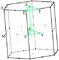
b.    LDA                      c.    LDA+DMFT

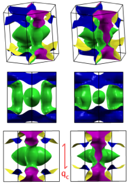
Figure 19: (Color online) (a) 1. BZ of the $Cmc2_{1}$ structure, including the high-symmetry lines used to plot the band structures. The $a^{*}$ axis runs towards M, the $b^{*}$ axis towards $Y$. (b column) LDA Fermi surface, and (c column) QP Fermi surface from LDA+DMFT. The second row of the columns show the BZ along $a^{*}$, the third row along $b^{*}$. In the latter column the experimental CDW nesting vector $\mathbf{q}_{c}$ is displayed.

To proceed it is important to realize that studying only the single high-symmetry line along $\Gamma$-Z in order to reveal a possible CDW instability may not be sufficient. In fact FS nesting can only be thoroughly investigated by taking into account the complete FS in the full BZ. With this aim we have plotted the LDA FS and the deformed LDA+DMFT FS in Fig. 19. In LDA the FS consists of two sheets which for the main part can truly be associated to $A_{1g}$ and $E_{g}$. The $A_{1g}$-like one shows the expected strong 1D behavior, i.e., corresponds to two main surfaces extending dominantly along ($k_{x}$,$k_{y}$), however with no real flattening. As already stated, the distance between these two surface parts is too large to account for the experimentally observed nesting. The second sheet incorporates the $E_{g2}$ electron pocket at $\Gamma$ as well as two $E_{g1}$ “pillars” on the $b^{*}$ axis (where also $\Gamma$-Y runs), extending along $c^{*}$ and opening towards the zone boundaries. Within LDA+DMFT the $E_{g2}$ pocket shrinks and the $E_{g1}$ pillars thicken. Interestingly, the first sheet is indeed only little modified in the immediate neighborhood of the $c^{*}$ axis, however the further parts along $a^{*}$ tend to flap down towards lower absolute values. Finally these latter parts are now not only within the distance of the experimental nesting vector ${\mathbf{q}}_{c}$=$0.5{\bf c}^{*}$, but are furthermore somehow more flattened. That this shift indeed brings these outer parts very close to half filling may be seen in Fig. 20. There the Wannier band-structure plot includes a line with non-high symmetry endpoints named “M/2” and “A/2”. These latter points are halfway from $\Gamma$ to M and halfway from Z to A (cf. Fig. 19). A true quantitative determination of the influence of the FS shape and of nesting properties on the CDW instability will require a full calculation of the Lindhard function using the presently calculated self-energy. Although it is conceivable that a truly accurate account of the CDW transition for this material would require going beyond a $\mathbf{k}$-independent self-energy, we feel that the interorbital charge transfer and corresponding FS deformation found in the present work qualitatively points to the correct mechanism.

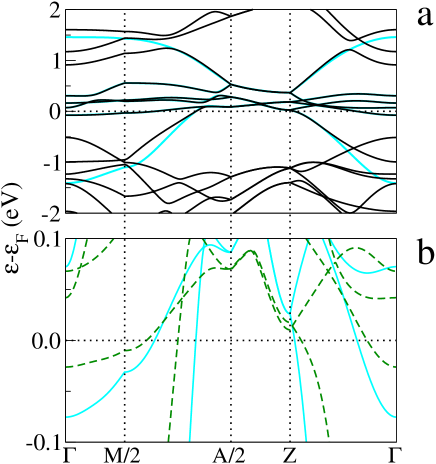
Figure 20: (Color online) (a) LDA band structure (dark) and according Wannier bands (cyan/light gray) along a closed path in the 1. BZ including the line connecting “M/2”and “A/2” (see text). (b) pure (cyan/light gray) and renormalized (darkgreen dashed/dark dashed) Wannier bands.

Let us finally comment on the role of the $E_{g}$ electrons in the MIT. It appears from our findings on the FS that the CDW in this material is in fact associated with the $A_{1g}$ electrons. The question then arises of the fate of the remaining $E_{g}$ electrons through the MIT. Of course, from a many-body viewpoint, and in view of our present and earlier results Lechermann et al. (2005a), one has to question the band-like character of these states from early on. The very narrow $E_{g}$ bandwidth causes a very low coherence scale for the corresponding QPs. Thus above $T_{\rm{MIT}}$ the $E_{g}$ QPs have not yet reached their coherence scale Lechermann et al. (2005a), which leaves them essentially localized already in the “metal”. In a sense, this is a realisation of an “orbital selective” phase Anisimov et al. (2002) at intermediate temperatures, i.e., a coexistence region of correlation-induced localized states and still itinerant states for $T$$>$$T_{\mbox{\tiny{MIT}}}$. In such a regime, the $A_{1g}$ electrons acquire a large scattering rate due to the presence of almost localized $E_{g}$ degrees of freedom, as studied in Refs. [Liebsch, 2005; Biermann et al., 2005]. This is a likely explanation of the “bad-metal” behavior observed above the MITLiebsch (2005); Biermann et al. (2005), and is also in good agreement with recent optical studies Kézsmárki et al. (2006). We also performed supporting two-site cluster-DMFT calculations, in order to allow for explicit intersite V-V self-energy terms, revealing no essential differences to the outlined picture. A closer investigation of the CDW state, i.e., the electronic structure of the system in the paramagnetic insulating regime below $T_{\rm{MIT}}$ is however necessary Fagot et al. (2005, 2006); Lechermann (to be published), including their spin degree of freedom, to reveal more details about the role of the $E_{g}$ elecrons.

IV Conclusion and prospects

In this paper, we have explored in detail the use of WFs as a flexible technique to perform electronic-structure calculations within the LDA+DMFT framework. WFs are useful for two different purposes. First, as a physically meaningful way of defining the correlated orbitals to which a many-body treatment will be applied. Second, as a convenient choice of basis functions for interfacing the many-body (DMFT) part of the calculation with virtually any kind of band-structure method. In this paper, three different methods have been used, namely a pseudopotential-based method (MBPP), an FLAPW method and an LMTO-based method. We have applied this approach to two transition-metal compounds. The first one, SrVO₃, was chosen in view of its simplicity as a testing ground for performing a detailed comparison between two different Wannier constructions: the maximally-localized-Wannier-function construction (MLWF) and the N-th order muffin-tin-orbital (NMTO) method. For this simple material, very close agreement between the two methods was found. The second material, BaVS₃, was chosen in view of its physical interest and of some open key questions. We have been able, in particular, to make new precise statements about the correlation-induced changes of the Fermi surface for this material, using our Wannier based method.

There are several directions in which the present work can be extended, and several open issues which need further attention. Here, we outline just a few of them. First, we emphasized above that the localisation properties of the Wannier functions depend of course on the energy range (or alternatively the set of bands) defining the subspace $\mathcal{W}$ in which the Wannier construction is performed. The correlated orbitals are then picked as a subset $\mathcal{C}$$\subseteq$$\mathcal{W}$, in general smaller than $\mathcal{W}$ itself. In the actual calculations performed in this paper, the minimal choice $\mathcal{C}$=$\mathcal{W}$ was made, associated for the two materials that were considered to exhibit low-energy bands with dominant $t_{2g}$ character. This of course, means that the correlated orbitals defining $\mathcal{C}$ had sizeable weights on ligand atoms. In contrast, one may want to enlarge $\mathcal{W}$ (including in particular ligand bands) and define the correlated subset from Wannier orbitals which would be more localized on the transition-metal site. Exploring these various choices, and comparing them to other choices in which the correlated orbitals are not constructed from WFs (e.g are taken to be heads of LMTOs, or truncated WFs, or even atomic wavefunctions) is certainly worth further investigations, particularly in the context of late transition-metal oxides. An important related issue is the appropriate way of calculating the local-interaction (Hubbard) parameters from first principles, for each of the possible choices of correlated orbitals. Working with WFs will make it easier to address this issue in a manner which is independent of the underlying band-structure method and basis set used for performing the calculations in practice. Finally, one should emphasize that the accuracy of the DMFT approximation depends on the choice made for the local orbitals defining $\mathcal{C}$. In fact, it has been recently suggested Paul and Kotliar (2006) that the local orbitals could be chosen in such a way as to make the DMFT approximation optimal (according to some criterion on the magnitude of the local interactions).

Another line of development that we are currently pursuing, is the practical implementation of the self-consistency over the charge density (and of total energy), along the lines of Appendix A, within non-LMTO based electronic structure methods. A more remote perspective for such developments would be the possibility of allowing for local structural relaxation for correlated materials within LDA+DMFT. Additionally, the Wannier-based formalism is also well suited for the calculation of response functions (e.g. optics). We hope to be able to address these issues in future work.

Appendix A Self-consistency over the charge density in LDA+DMFT

In this appendix, we briefly discuss the implementation of self-consistency over the charge density in the LDA+DMFT framework. Until now, this has been implemented in practice only in the MTO Savrasov et al. (2001); Chioncel et al. (2003); Savrasov and Kotliar (2004); Pourovskii et al. (to be published) or KKR Minár et al. (2005) context. Here, we discuss the use of other basis sets, with particularly the Wannier framework in mind.

As outlined in section (II.1.4), charge self-consistency means that the KS cycle and the DMFT loop are explicitly coupled, i.e., the charge density is calculated at the end of a DMFT cycle (including self-energy effects). From the new charge density, a new KS potential is obtained, and so on.

The charge density is calculated from the full Green’s function of the solid. Without yet introducing a specific basis set, it is given by Eq. (13), namely:

$$\rho(\mathbf{r})=\frac{1}{\beta}\sum_{n}\left\langle\mathbf{r}\left|\left[i\omega_{n}+\mu+\frac{\nabla^{2}}{2}-\hat{V}_{\rm{KS}}-\Delta\hat{\Sigma}\right]^{-1}\right|\mathbf{r}\right\rangle\mbox{e}^{i\omega_{n}0^{+}}\,.$$ (31)

We shall find it convenient to split $\rho(\mathbf{r})$ into

$$\rho(\mathbf{r}) = \rho_{\rm{KS}}(\mathbf{r})+\left[\rho(\mathbf{r})-\rho_{\rm{KS}}(\mathbf{r})\right]$$ (33)

$$\equiv \rho_{\rm{KS}}(\mathbf{r})+\Delta\rho(\mathbf{r})\quad,$$

$$\mbox{with}\quad\rho_{\rm{KS}}(\mathbf{r})=\left\langle\mathbf{r}\left|\hat{G}_{\rm{KS}}\right|\mathbf{r}\right\rangle\quad.$$

It is important to realize here that the demand for charge neutrality is not imposed on $\rho_{\rm{KS}}(\mathbf{r})$ but rather on $\rho(\mathbf{r})$. The chemical potential $\mu$ must be therefore explicitly determined (at the end of a DMFT loop) in such a way that the total number of electrons is the correct one (i.e. charge neutrality is preserved): $N_{e}$=$\mbox{tr}\,\hat{G}$=$\int d\mathbf{r}\rho(\mathbf{r})$. This value of the chemical potential will in general not be such that $\mbox{tr}\,\hat{G}_{\rm{KS}}$=$\int d\mathbf{r}\rho_{\rm{KS}}(\mathbf{r})$ equals the total number of electrons $N_{e}$. This is quite natural, since the KS representation of the charge density by independent KS wavefunctions no longer holds in the LDA+DMFT formalism.

Formally, the charge-density correction $\Delta\rho$ may be expressed as

$$\Delta\rho(\mathbf{r}) = \left\langle\mathbf{r}\left|\hat{G}-\hat{G}_{\rm{KS}}\right|\mathbf{r}\right\rangle$$ (34)

$$= \left\langle\mathbf{r}\left|\hat{G}_{\rm{KS}}\left(\hat{G}_{\rm{KS}}^{-1}-\hat{G}^{-1}\right)\hat{G}\right|\mathbf{r}\right\rangle$$

$$= \left\langle\mathbf{r}\left|\hat{G}_{\rm{KS}}\,\hat{\Delta\Sigma}\,\hat{G}\right|\mathbf{r}\right\rangle\quad.$$

In a concrete implementation, this equation must be written in the specific basis set of interest. We shall do this with the Wannier formalism in mind, i.e. use the basis functions (19) corresponding to the set $\mathcal{W}$, which are unitarily related to the Bloch functions by

$$|w_{\mathbf{k}\alpha}\rangle\equiv\sum_{{\mathbf{T}}}\mbox{e}^{i\mathbf{k}\cdot\mathbf{T}}|w_{\mathbf{T}\alpha}\rangle=\sum_{\nu\in\,{\cal W}}U_{\alpha\nu}^{(\mathbf{k})}|\psi^{\hfill}_{{\mathbf{k}}\nu}\rangle\,.$$ (35)

Since in the Wannier basis set $\mathbf{G}_{\rm{KS}}$ and $\mathbf{G}$ are block diagonal, they have common non-zero matrix elements only in the chosen subspace $\mathcal{W}$. Let us define the operator $\Delta\hat{N}$ in $\mathcal{W}$ by its matrix elements:

$$\Delta N_{\alpha\alpha^{\prime}}^{(\mathbf{k})}\equiv\frac{1}{\beta}\sum_{n\,mm^{\prime}}G_{\alpha m}^{\rm{KS}}(\mathbf{k},i\omega_{n})\,\Delta\Sigma_{mm^{\prime}}(i\omega_{n})\,G_{m^{\prime}\alpha^{\prime}}(\mathbf{k},i\omega_{n})\,,$$ (36)

Note that the indices $\alpha\alpha^{\prime}$ run over $\mathcal{W}$, while the summation over $mm^{\prime}$ runs only within the correlated subset $\mathcal{C}$. Note also that the frequncy summation in this expression converges rather quickly, since the terms in the sum decay as $1/\omega_{n}^{2}$ at large frequencies (hence no convergence factor e${}^{i\omega_{n}0^{+}}$ is needed in the sum). The desired charge-density correction therefore reads:

$$\Delta\rho(\mathbf{r})=\sum_{\mathbf{k}\alpha\alpha^{\prime}}\langle\mathbf{r}|w_{\mathbf{k}\alpha}\rangle\,\Delta N_{\alpha\alpha^{\prime}}^{(\mathbf{k})}\langle w_{\mathbf{k}\alpha^{\prime}}|\mathbf{r}\rangle\,$$ (37)

Alternatively, (37) can also be written in the Bloch basis as:

$$\Delta\rho(\mathbf{r})=\sum_{\mathbf{k}}\sum_{\nu\nu^{\prime}\in\mathcal{W}}\psi^{\hfill}_{\mathbf{k}\nu}(\mathbf{r})\psi_{\mathbf{k}\nu^{\prime}}^{*}(\mathbf{r})\,\Delta N_{\nu\nu^{\prime}}^{(\mathbf{k})}\,,$$ (38)

$$\mbox{with}\quad\Delta N_{\nu\nu^{\prime}}^{(\mathbf{k})}=\sum_{\alpha\alpha^{\prime}}U^{(\mathbf{k})}_{\nu\alpha}\,\Delta N_{\alpha\alpha^{\prime}}^{(\mathbf{k})}\,U^{(\mathbf{k})*}_{\alpha^{\prime}\nu^{\prime}}$$ (39)

The KS part of the charge density is easily calculated within the given band-structure code:

$$\rho_{\rm{KS}}(\mathbf{r})=\mathop{\sum_{\mathbf{k}\nu}}_{\varepsilon_{\mathbf{k}\nu}\leq\mu}|\psi^{\hfill}_{{\mathbf{k}}\nu}(\mathbf{r})|^{2}\quad.$$ (40)

Note the difference between (38) and (40), as in (38) additional terms, off-diagonal in the band indices, contribute to $\Delta\rho(\mathbf{r})$. In this respect it proves to be convenient to introduce the density matrix of KS orbitals:

$$D_{\nu^{\prime}\nu}^{(\mathbf{k})}(\mathbf{r})=\psi^{\hfill}_{\mathbf{k}\nu}(\mathbf{r})\psi^{*}_{\mathbf{k}\nu^{\prime}}(\mathbf{r})\,,$$ (41)

The two contributions to the charge-density may now be compactly written as:

$$\rho_{\rm{KS}}(\mathbf{r}) = \mathop{\sum_{\mathbf{k}\nu}}_{\varepsilon_{\mathbf{k}\nu}\leq\mu}D^{(\mathbf{k})}_{\nu\nu}(\mathbf{r})\quad,$$ (42)

$$\Delta\rho(\mathbf{r}) = \sum_{\mathbf{k}}\mbox{tr}\,_{\nu}\left[\mathbf{D}^{(\mathbf{k})}\cdot{\bf\Delta N}^{(\mathbf{k})}\right]\quad.$$ (43)

Hence finally, we can write the full charge density, i.e., eq. (31), in the following explicit form:

$$\rho(\mathbf{r})=\sum_{\mathbf{k}\nu\nu^{\prime}}D_{\nu^{\prime}\nu}^{(\mathbf{k})}(\mathbf{r})\Delta N^{(\mathbf{k})}_{\nu\nu^{\prime}}+\sum_{\nu}\Theta(\mu-\varepsilon_{\mathbf{k}\nu})D_{\nu\nu}^{(\mathbf{k})}(\mathbf{r})\,.$$ (44)

Generalization to finite-$T$ DFT is straightforward. Realize that in the Wannier implementation, the first (double) sum in (44) would only run over Bloch bands in the $\mathcal{W}$ set (since only there $\Delta N$ is non-zero), while the second sum runs over all filled Bloch states. Again, it is important that the chemical potential has been correctly updated at the end of the DMFT loop, so that the full charge density (44) sums up to the correct total number of electrons, hence insuring charge neutrality.

Expression (44) has in fact a general degree of validity, not limited to the Wannier implementation, provided the matrix $\Delta N$, originally calculated in the basis set in which the DMFT calculation has been performed, is correctly transformed to the Bloch basis set.

Appendix B Free-energy functional and total energy

For the sake of completeness, we briefly summarize in this appendix how the LDA+DMFT formalism for electronic structure, described in Sec. II can be derived from a free-energy functional. As pointed out by Savrasov and Kotliar Savrasov and Kotliar (2004), a (“spectral-density-”) functional of both the electron charge density $\rho(\mathbf{r})$ and the on-site Green’s function in the correlated subset $G^{\rm{loc}}_{mm^{\prime}}$, can be constructed for this purpose. Let us emphasize that these are independent quantities: because $\mathbf{G}_{\rm{loc}}$ is restricted to on-site components and to the correlated subset $\mathcal{C}$, the charge density $\rho(\mathbf{r})$ cannot be reconstructed from it. A compact formula for the total energy can also be obtained from this functional formulation Amadon et al. (2006); Georges (2004); Savrasov and Kotliar (2004), given at the end of this appendix.

The functional is constructed by introducing source terms $V_{\rm{KS}}(\mathbf{r})$$-$$V_{\rm{ext}}(\mathbf{r})$ and $\Delta\Sigma_{mm^{\prime}}(i\omega_{n})$, coupling to the operators $\hat{\psi}^{\dagger}(\mathbf{r})\hat{\psi}(\mathbf{r})$ and $\sum_{\mathbf{T}}\chi^{*}_{m}(\mbox{$\mathbf{r}$$-$$\mathbf{R}$$-$$\mathbf{T}$})\hat{\psi}(\mathbf{r},\tau)\hat{\psi}^{\dagger}(\mathbf{r}^{\prime},\tau^{\prime})\chi_{m^{\prime}}(\mbox{$\mathbf{r}^{\prime}$$-$$\mathbf{R}$$-$$\mathbf{T}$})$, respectively. It reads:

$$\Omega[\rho,G^{loc}_{mm^{\prime}};V_{\rm{KS}},\Delta\Sigma_{mm^{\prime}}]=$$ (45)

$$-\frac{1}{\beta}\rm{tr}\ln\left[i\omega_{n}+\mu+\frac{\nabla^{2}}{2}-\hat{V}_{\rm{KS}}-\Delta\hat{\Sigma}\right]$$

$$-\int d\mathbf{r}\,\left(V_{\rm{KS}}(\mathbf{r})-V_{\rm{ext}}(\mathbf{r})\right)\rho(\mathbf{r})-\rm{tr}[\hat{G}_{loc}\Delta\hat{\Sigma}]$$

$$+\frac{1}{2}\int d\mathbf{r}d\mathbf{r}^{\prime}\frac{\rho(\mathbf{r})\rho(\mathbf{r}^{\prime})}{|\mathbf{r}-\mathbf{r}^{\prime}|}+E_{\rm{xc}}[\rho]$$

$$+\sum_{\mathbf{T}}\left(\Phi_{\rm{imp}}[G^{loc}_{mm^{\prime}}]-\Phi_{\rm{DC}}[G^{loc}_{mm^{\prime}}]\right)$$ (46)

In this expression, $\Phi_{\rm{imp}}$ is the Luttinger-Ward functional of the quantum impurity model, and $\Phi_{\rm{DC}}$ a corresponding functional generating the double-counting correction. Note that, as usual, it is understood that $\Delta\hat{\Sigma}$ in the logarithm term of (46) represents the self-energy correction on the lattice.

Variations of this functional with respect to the sources $\delta\Omega/\delta\,V_{\rm{KS}}$=0 and $\delta\Omega/\delta\Sigma_{mm^{\prime}}$=0 yield the standard expression of the charge density and local Green’s function in terms of the full Green’s function in the solid, Eq. (2). The Legendre multiplier functions $V_{\rm{KS}}$ and $\Delta\Sigma$ can be eliminated in terms of $\rho$ and $G_{\rm{loc}}$, so that a functional only of the local observables is obtained:

$$\Gamma[\rho,G_{\rm{loc}}]=\Omega\left[\rho,G^{loc}_{mm^{\prime}};V_{\rm{KS}}[\rho,G_{\rm{loc}}],\Delta\Sigma[\rho,G_{\rm{loc}}]\right]\,.$$ (47)

Extremalization of this functional with respect to $\rho$ ($\delta\Gamma/\delta\rho$=0) and $G_{\rm{loc}}$ ($\delta\Gamma/\delta\,G_{\rm{loc}}$=0) yields the expression of the KS potential and self-energy correction at self-consistency, i.e., the self-consistency conditions (over both the local projected Green’s function and the charge density) of the LDA+DMFT formalism.

Using the above expressions, the free-energy can be written as:

$$\Omega= \Omega_{\rm{DFT}}+\mbox{tr}\,\ln\,\hat{G}_{\rm{KS}}^{-1}-\mbox{tr}\,\ln\,\hat{G}^{-1}-\mbox{tr}\,[\hat{G}_{\rm{loc}}\hat{\Sigma}_{\rm{imp}}]$$ (48)

$$+\mbox{tr}\,[\hat{G}_{\rm{loc}}\hat{\Sigma}_{\rm{DC}}]+\sum_{\mathbf{T}}\left(\Phi_{\rm{imp}}-\Phi_{\rm{DC}}\right)\,.$$

In this expression, $\Omega_{\rm{DFT}}$ is the usual density-functional theory expression of the free-energy (calculated at the self-consistent LDA+DMFT charge density, however). Taking the zero-temperature limit of this expression leads to the following expression Amadon et al. (2006); Savrasov and Kotliar (2004) of the total energy at $T$=0:

$$E_{\rm{LDA+DMFT}}= E_{\rm{DFT}}+\langle\hat{H}_{U}\rangle-E_{\rm{DC}}$$ (49)

$$+\sum_{\mathbf{k}\alpha\alpha^{\prime}}H^{\rm{KS}}_{\alpha\alpha^{\prime}}(\mathbf{k})\left[\langle\hat{c}^{\dagger}_{\mathbf{k}\alpha}\hat{c}^{\hfill}_{\mathbf{k}\alpha^{\prime}}\rangle_{\rm{DMFT}}-\langle\hat{c}^{\dagger}_{\mathbf{k}\alpha}\hat{c}^{\hfill}_{\mathbf{k}\alpha^{\prime}}\rangle_{\rm{KS}}\right]$$

Note that $\alpha,\alpha^{\prime}$ cover the full electronic Hilbert space. Finally, it should be understood that in deriving the LDA+DMFT equations from this free-energy functionals, we have implicitly assumed that the orbitals $\chi_{m}$ defining the correlated subset $\mathcal{C}$ were kept fixed. In practice however, one may want also to optimze these orbitals, e.g. by minimizing the free-energy $\Omega$. Furthermore, we emphasize that in the implementation of the charge self-consistency described in Appendix A, it was explicitly assumed that these orbitals were recalculated as Wannier functions associated with the new KS potential. This is done at each stage of the iteration over the charge density. If instead the local orbitals are frozen (e.g. from the LDA potential), then they are no longer unitarily related to the new set of KS orbitals corresponding to the new potential, and the formulas derived in Appendix A have to be appropriately reconsidered.

Appendix C Technical details

In the following we provide further details on the band-structure calculations performed in this work. Concerning the computations using the MBPP code, due to the significant ionic character of the treated compounds, the semicore states of Ba, Sr and V were treated as valence. Hence the pseudopotentials were constructed for Sr(($4s4p4d$)/Ba($5s5p5d$), V($3s3p3d$) and O(($2s2p2d$)/S(($3s3p3d$). The partial-core correction was used in all constructions. In the crystal calculations, localized functions were introduced for all valence states. Thereby, the localized functions are atomic pseudo wavefunctions, either multiplied with a cut-off function ($sd$) or minus a spherical Bessel function ($p$). The cut-off radius for the V($3d$) local functions was chosen as 2.0 a.u.. The plane-wave cutoff energy $E_{\rm{pw}}^{\rm{(cut)}}$ was 24 Ryd for SrVO₃ and 20 Ryd for BaVS₃, and the Perdew-Wang exchange-correlation functional Perdew and Wang (1992) was used in all calculations.

In the FLAPW calculation for SrVO₃, the atomic-sphere radii for Sr, V, and O were chosen to be 2.5, 2.0, and 1.55 a.u., respectively and the FLAPW basis size was set to include all plane waves up to $E_{\rm{pw}}^{\rm{(cut)}}$=20.25 Ryd . The local orbitals sector of the basis was used to include the high lying V($3s$), V($3p$), Sr($4s$), Sr($4p$) and O($2s$) core states as valence states in the calculations. Additional V($3d$) local orbitals were used to relax the linearization of the transition metal $d$-bands. The Hedin-Lundquist exchange-correlation functional Hedin and Lundquist (1971) was used in the calculation.

For the self-consistent LMTO calculation of the effective LDA potential for SrVO₃ we have used the prescription described in Ref. [Pavarini et al., 2005]. The radii of potential spheres were chosen to be 3.46 a.u., 2.3 a.u. and 2.04 a.u. for Sr, V and O atoms, respectively. Twelve empty spheres were introduced above the octahedron edges with the radii 1.01 a.u. The LMTO basis set used in the calculation were $s(p)d(f)$, $spd$, $(s)p(d)$ and $s(p)(d)$ for Sr, V, O and empty spheres, respectively. $(l)$ means that the $l$-partial waves were downfolded within TB-LMTO-ASA. The von Barth-Hedin exchange-correlation functional von Barth and Hedin (1972) was used in the calculation, which is very similar to the Hedin-Lundquist parametrization. These elder $E_{\rm{xc}}$ representations utilize the same interpolation formula.

The construction of the MLWFs from the disentangling procedure for BaVS₃ was described in section III.2.3. In the case of SrVO₃, no energy windows have to be defined, since the $t_{2g}$-like bands form an isolated group of bands. The NMTO-WFs for SrVO₃ were obtained by imposing that for a $t_{2g}$ orbital, the $t_{2g}$ character on any other V site must vanish. We used $N$=2 and chose the energies for which this quadratic MTO set is complete as: $\epsilon_{0}$=-1.29 eV, $\epsilon_{1}$=0 eV and $\epsilon_{2}$=1.61 eV with respect to Fermi level. Finally, the NMTO set was symmetrically orthonormalized.