Virial coefficients and osmotic pressure in polymer solutions
in good-solvent conditions

Abstract

We determine the second, third, and fourth virial coefficients appearing in the density expansion of the osmotic pressure $\Pi$ of a monodisperse polymer solution in good-solvent conditions. Using the expected large-concentration behavior, we extrapolate the low-density expansion outside the dilute regime, obtaining the osmotic pressure for any concentration in the semidilute region. Comparison with field-theoretical predictions and experimental data shows that the obtained expression is quite accurate. The error is approximately 1-2% below the overlap concentration and rises at most to 5-10% in the limit of very large polymer concentrations.

PACS: 61.25.Hq, 82.35.Lr

I Introduction

For sufficiently high molecular weights, dilute and semidilute polymer solutions under good-solvent conditions exhibit a universal scaling behavior.[1, 2, 3, 4] For instance, the radius of gyration $R_{g}$, which gives the average size of the polymer, scales as $N^{\nu}$, where $N$ is the degree of polymerization and $\nu$ a universal exponent, $\nu\approx 0.5876$ (Ref. [5]). The osmotic pressure $\Pi$ is one of the most easily accessible quantities in polymer physics. When $N$ is large, it obeys a general scaling law[2, 3, 4] (here and in the following we only consider monodisperse solutions)

$$Z\equiv{M\Pi\over RT\rho}={\Pi\over k_{B}Tc}=f(cR_{g}^{3}),$$ (1)

where $c$ is the polymer number density, $\rho$ the ponderal concentration, $M$ the molar mass of the polymer, and $T$ the absolute temperature. The function $f(x)$ is universal, so that the determination of $Z$ in a specific model allows one to predict $\Pi$ for any polymer solution. In the dilute limit the compressibility factor $Z$ can be expanded in powers of $c$ obtaining[6]

$$Z=1+\sum_{n=1}B_{n+1}c^{n},$$ (2)

where the coefficients $B_{n}$ are knows as virial coefficients. Knowledge of $B_{n}$ allows one to compute $\Pi$ in the dilute regime in which $cR^{3}_{g}\ll 1$. The coefficients $B_{n}$ depend on the polymer solution. Eq. (2) can be rewritten as

$$Z=1+\sum_{n=1}A_{n+1}(cR_{g}^{3})^{n}\qquad\qquad A_{n+1}\equiv B_{n+1}R_{g}^{-3n},$$ (3)

where $R_{g}$ is the zero-density radius of gyration of the polymer. The general scaling law (1) implies that for $N\to\infty$ the coefficients $A_{n+1}$ approach universal constants $A_{n+1}^{*}$ that are independent of chemical details. The value of $A_{2}^{*}$ has been the object of many theoretical studies (sometimes, the interpenetration radius $\Psi\equiv 2(4\pi)^{-3/2}A_{2}$ is quoted instead of $A_{2}$). The most precise estimates have been obtained by means of Monte Carlo (MC) simulations: $A^{*}_{2}=5.494\pm 0.005$ (Ref. [7]), $A^{*}_{2}=5.504\pm 0.007$ (Ref. [8]), $A^{*}_{2}=5.490\pm 0.027$ (Ref. [9]). Eq. (1) is only valid for high molecular weights. Since in many cases $N$ is not very large, it is important to consider also the leading correction to this expression. As predicted by the renormalization group and extensively verified numerically, for $N$ large but finite we have

$$Z\approx f(cR^{3}_{g})+{a_{2}\over N^{\Delta}}g(cR^{3}_{g}),\qquad\qquad A_{n+1}\equiv{B_{n+1}\over R^{3n}_{g}}\approx A_{n+1}^{*}+{a_{2}b_{n+1}\over N^{\Delta}},$$ (4)

where $b_{2}=1$, $\Delta$ is a universal exponent whose best estimate is[10] $\Delta=0.515\pm 0.007^{+0.010}_{-0.000}$, and, of course, $g(x)=1+\sum b_{n+1}x^{n}$. The function $g(x)$ as well as the constants $b_{n}$ are universal. All chemical details as well as polymer properties—for instance, the temperature—are encoded in a single constant $a_{2}$ that varies from one polymer solution to the other. In this paper we extend the previous calculations to the third and fourth virial coefficient, computing $A_{3}^{*}$, $A_{4}^{*}$, and $b_{3}$. For this purpose we perform an extensive MC simulation of the lattice Domb-Joyce model,[11] considering walks of length varying between 100 and 8000 and three different penalties for the self-intersections.

Knowledge of the first virial coefficients and of the leading scaling corrections allows us to obtain a precise prediction for the osmotic pressure in the dilute regime (the expression is apparently accurate up to $B_{2}c\approx 1$), even for relatively small values of the degree of polymerization. Finite-length effects are taken into account by properly tuning a single nonuniversal parameter. Once the virial expansion is known, we can try to resum it to obtain an interpolation formula that is valid in the semidilute regime. We will show that a simple expression that takes into account the large-density behavior of $Z$ provides a good approximation to $Z$, even outside the dilute regime.

The paper is organized as follows. In Sec. II we derive the virial expansion for a polymer solution. In Sec. III we define the model, while in Sec. IV we compute the universal constants defined above that are associated with the virial coefficients. In Sec. V we present our conclusions and, in particular, give an interpolation formula for $Z$ that is also valid in the semidilute regime. Some technical details are presented in the Appendix.

II Virial expansion

We wish now to derive the virial expansion for a polymer solution. Such an expansion is easily derived in the grand-canonical ensemble.[12] For this purpose, we first define the configurational partition function $Q_{L}$ of $L$ polymers in a volume $V$:

$$Q_{L} = \int d\mu\,\exp\left(-\beta\sum_{i<j}V_{ij}^{\rm inter}\right)$$ (5)

$$d\mu = \left[\prod_{i\alpha}d^{3}{\mathbf{r}}_{\alpha i}\right]\exp\left(-\beta\sum_{i}V_{i}^{\rm intra}\right),$$ (6)

where $V_{ij}^{\rm inter}$ is the sum of all terms of the Hamiltonian that correspond to interactions of monomers belonging to two different polymers $i$ and $j$, $V_{i}^{\rm intra}$ is the contribution due to interactions of monomers belonging to the same polymer $i$, and ${\mathbf{r}}_{\alpha i}$ is the position of monomer $\alpha$ belonging to polymer $i$. Then, we set

$$\Xi=\sum_{L}{z^{L}\over L!}Q_{L}.$$ (7)

The virial expansion is obtained by performing an expansion in powers of $z$. We introduce the Mayer function

$$f_{ij}\equiv\exp(-\beta V_{ij}^{\rm inter})-1$$ (8)

and define the following integrals:

$$I_{2} \equiv \int d^{3}{\mathbf{r}}_{12}\,\langle f_{12}\rangle_{{\mathbf{0}},{\mathbf{r}}_{12}}$$ (9)

$$I_{3} \equiv \int d^{3}{\mathbf{r}}_{12}d^{3}{\mathbf{r}}_{13}\left\langle f_{12}f_{13}f_{23}\right\rangle_{{\mathbf{0}},{\mathbf{r}}_{12},{\mathbf{r}}_{13}}$$ (10)

$$I_{4} \equiv \int d^{3}{\mathbf{r}}_{12}d^{3}{\mathbf{r}}_{13}d^{3}{\mathbf{r}}_{14}\left\langle f_{12}f_{23}f_{34}f_{14}(3+6f_{13}+f_{13}f_{24})\right\rangle_{{\mathbf{0}},{\mathbf{r}}_{12},{\mathbf{r}}_{13},{\mathbf{r}}_{14}}$$ (11)

$$T_{1} \equiv \int d^{3}{\mathbf{r}}_{12}d^{3}{\mathbf{r}}_{13}\left\langle f_{12}f_{13}\right\rangle_{{\mathbf{0}},{\mathbf{r}}_{12},{\mathbf{r}}_{13}}-\left[\int d^{3}{\mathbf{r}}_{12}\left\langle f_{12}\right\rangle_{{\mathbf{0}},{\mathbf{r}}_{12}}\right]^{2}$$ (12)

$$T_{2} \equiv \int d^{3}{\mathbf{r}}_{12}d^{3}{\mathbf{r}}_{13}d^{3}{\mathbf{r}}_{14}\left\langle f_{12}f_{13}f_{14}\right\rangle_{{\mathbf{0}},{\mathbf{r}}_{12},{\mathbf{r}}_{13},{\mathbf{r}}_{14}}-\left[\int d^{3}{\mathbf{r}}_{12}\left\langle f_{12}\right\rangle_{{\mathbf{0}},{\mathbf{r}}_{12}}\right]^{3}$$ (13)

$$T_{3} \equiv \int d^{3}{\mathbf{r}}_{12}d^{3}{\mathbf{r}}_{13}d^{3}{\mathbf{r}}_{14}\left\langle f_{12}f_{23}f_{34}\right\rangle_{{\mathbf{0}},{\mathbf{r}}_{12},{\mathbf{r}}_{13},{\mathbf{r}}_{14}}-\left[\int d^{3}{\mathbf{r}}_{12}\left\langle f_{12}\right\rangle_{{\mathbf{0}},{\mathbf{r}}_{12}}\right]^{3}$$ (14)

$$T_{4} \equiv \int d^{3}{\mathbf{r}}_{12}d^{3}{\mathbf{r}}_{13}d^{3}{\mathbf{r}}_{14}\left\langle f_{12}f_{23}f_{13}f_{34}\right\rangle_{{\mathbf{0}},{\mathbf{r}}_{12},{\mathbf{r}}_{13},{\mathbf{r}}_{14}}$$ (16)

$$-\left[\int d^{3}{\mathbf{r}}_{12}\left\langle f_{12}\right\rangle_{{\mathbf{0}},{\mathbf{r}}_{12}}\right]\left[\int d^{3}{\mathbf{r}}_{12}d^{3}{\mathbf{r}}_{13}\left\langle f_{12}f_{13}f_{23}\right\rangle_{{\mathbf{0}},{\mathbf{r}}_{12},{\mathbf{r}}_{13}}\right].$$

Here $\langle\cdot\rangle_{{\mathbf{0}},{\mathbf{r}}}$ indicates an average over two independent polymers such that the first one starts at the origin and the second starts in ${\mathbf{r}}$. Analogously $\langle\cdot\rangle_{{\mathbf{0}},{\mathbf{r}}_{2},{\mathbf{r}}_{3}}$ and $\langle\cdot\rangle_{{\mathbf{0}},{\mathbf{r}}_{2},{\mathbf{r}}_{3},{\mathbf{r}}_{4}}$ refer to averages over three and four polymers respectively, the first one starting in the origin, the second in ${\mathbf{r}}_{2}$, etc.

Then, a simple calculation gives

$${\beta\Pi}={1\over V}\ln\Xi = z+{z^{2}\over 2}I_{2}+{z^{3}\over 6}(I_{3}+3T_{1}+3I_{2}^{2})$$ (18)

$$+{z^{4}\over 24}(I_{4}+4T_{2}+12T_{3}+12T_{4}+16I_{2}^{3}+12I_{2}I_{3})+O(z^{5}).$$

The density is obtained by using

$$c=z{\partial\beta\Pi\over\partial z}.$$ (19)

The previous equation can be inverted to obtain $z$ in powers of $c$. Substituting in Eq. (18), we obtain expansion (2) with

$$B_{2} = -{1\over 2}I_{2},$$ (20)

$$B_{3} = -{1\over 3}I_{3}-T_{1},$$ (21)

$$B_{4} = -{1\over 8}I_{4}-{1\over 2}T_{2}-{3\over 2}T_{3}-{3\over 2}T_{4}+{9\over 2}I_{2}T_{1}.$$ (22)

Note that there are additional contributions to $B_{3}$ and $B_{4}$ which are missing in simple fluids.[12] Indeed, for a monoatomic fluid $T_{n}=0$. These terms are instead present in the polymer virial expansion.

In the following we shall consider a lattice model for polymers. In this case, the previous expressions must be trivially modified, replacing each integral with the corresponding sum over all lattice points.

III Model and observables

Since we are interested in computing the universal quantities $A_{n}^{*}$ and $b_{n}$, we can use any model that captures the basic polymer properties. For computational convenience we consider a lattice model. A polymer of length $N$ is modelled by a random walk $\{{\mathbf{r}}_{0},{\mathbf{r}}_{1},\ldots,{\mathbf{r}}_{N}\}$ with $|{\mathbf{r}}_{\alpha}-{\mathbf{r}}_{\alpha+1}|=1$ on a cubic lattice. To each walk we associate a Boltzmann factor

$$e^{-\beta H}=e^{-w\sigma},\qquad\qquad\sigma=\sum_{0\leq\alpha<\beta\leq N}\delta_{{\mathbf{r}}_{\alpha},{\mathbf{r}}_{\beta}},$$ (23)

with $w\geq 0$. The factor $\sigma$ counts how many self-intersections are present in the walk. This model is similar to the standard self-avoiding walk (SAW) model in which polymers are modelled by random walks in which self-intersections are forbidden. The SAW model is obtained for $w=+\infty$. For finite positive $w$ self-intersections are possible although energetically penalized. For any positive $w$, this model—hereafter we will refer to it as Domb-Joyce (DJ) model—has the same scaling limit of the SAW model[11] and thus allows us to compute the universal scaling functions that are relevant for polymer solutions. The DJ model has been extensively studied numerically in Ref. [10]. There, it was also shown that there is a particular value of $w$, $e^{-w^{*}}\approx 0.603$ (i.e., $w^{*}\approx 0.505838$), for which corrections to scaling with exponent $\Delta$ vanish: the nonuniversal constant $a_{2}$ is zero for $w=w^{*}$. Thus, simulations at $w=w^{*}$ are particularly convenient since the scaling limit can be observed for smaller values of $N$.

In the simulations we measure the virial coefficients using Eqs. (20), (21), and (22). In this model the Mayer function is simply

$$f_{ij}=e^{-\beta V_{ij}^{\rm inter}}-1=e^{-w\sigma_{ij}}-1$$ (24)

$$\sigma_{ij}=\sum_{\alpha\beta}\delta_{{\mathbf{r}}_{\alpha i},{\mathbf{r}}_{\beta j}}.$$ (25)

Here ${\mathbf{r}}_{\alpha i}$ is the position of monomer $\alpha$ of polymer $i$. The DJ model can be efficiently simulated by using the pivot algorithm.[13, 14, 15, 16] For the SAW an efficient implementation is discussed in Ref. [17]. The extension to the DJ model is straightforward, the changes in energy being taken into account by means of a Metropolis test. Such a step should be included carefully in order not to loose the good scaling behavior of the CPU time per attempted move. We use here the implementation discussed in Ref. [18]. The virial coefficients have been computed by using a simple generalization of the hit-or-miss algorithm discussed in Ref. [8]. Some details are reported in the Appendix.

IV Monte Carlo determination of the virial coefficients

We perform three sets of simulations at $w=0.375$, 0.505838, 0.775, using walks with $100\leq N\leq 8000$. Results are reported in Tables I, II, and III. As expected, the results for $w=0.505838$ are the least dependent on $N$, confirming that for this value of $w$ scaling corrections are very small. On the other hand, for $w=0.375$ and $w=0.775$ scaling corrections are sizable.

The numerical data are analyzed as discussed in Ref. [7]. We assume that $A_{n}$ has an expansion of the form

$$A_{n}(N,w)\approx A_{n}^{*}+{a_{n}(w)\over N^{\Delta}}+{c_{n}(w)\over N^{\Delta_{2,\rm eff}}}\;.$$ (26)

For $\Delta$ we use the best available estimate: $\Delta=0.515\pm 0.007^{+0.010}_{-0.000}$ (Ref. [10]). The term $1/N^{\Delta_{2,\rm eff}}$ should take into account analytic corrections behaving as $1/N$, and nonanalytic ones of the form $N^{-2\Delta}$, $N^{-\Delta_{2}}$ ($\Delta_{2}$ is the next-to-leading correction-to-scaling exponent). As discussed in Ref. [7], one can lump all these terms into a single one with exponent $\Delta_{2,\rm eff}=1.0\pm 0.1$. In order to estimate $A_{2}$ we also use the results that appear in Table 1 of Ref. [7] that refer to MC simulations of interacting SAWs.[19] A combined fit of the results for $A_{2}$ (with $1+5\times 2=11$ free parameters) gives

$$A_{2}^{*}=5.4986\pm 0.0010\pm 0.0002 \qquad\qquad N_{\rm min}=250,$$ (27)

$$A_{2}^{*}=5.4997\pm 0.0017\pm 0.0002 \qquad\qquad N_{\rm min}=500,$$ (28)

$$A_{2}^{*}=5.5013\pm 0.0030\pm 0.0003 \qquad\qquad N_{\rm min}=1000\;.$$ (29)

In each fit we have considered only the data with $N\geq N_{\rm min}$. We do not show results for $N_{\rm min}=100$ since in this case the fit has a somewhat large $\chi^{2}$. We report two error bars. The first one is the statistical error while the second gives the variation of the estimate as $\Delta$ and $\Delta_{2,\rm eff}$ vary within one error bar. The results show a small upward trend which is in any case of the order of the statistical errors. As our final estimate we quote

$$A_{2}^{*}=5.500\pm 0.003.$$ (30)

Note that in the polymer literature one often considers the interpenetration ratio $\Psi\equiv 2(4\pi)^{-3/2}A_{2}$ instead of $A_{2}$. We have

$$\Psi^{*}=2(4\pi)^{-3/2}A_{2}^{*}=0.24693\pm 0.00013.$$ (31)

The same analysis—but in this case we only rely on the DJ results—can be repeated for $A_{3}$. Estimates of $A_{3}$ are reported in Table II. The contribution proportional to $I_{3}$ appearing in Eq. (21)—the only one present in simple fluids— accounts for most of the result since the contribution proportional to $T_{1}$ is small, $T_{1}R_{g}^{-6}\approx 0.84$ in the scaling limit. Still in a high-precision calculation, $T_{1}$ cannot be neglected, giving a 9% correction. A fit of the results to Eq. (26) gives

$$A_{3}^{*}=9.788\pm 0.005\pm 0.002 \qquad\qquad N_{\rm min}=100,$$ (32)

$$A_{3}^{*}=9.786\pm 0.008\pm 0.001 \qquad\qquad N_{\rm min}=250,$$ (33)

$$A_{3}^{*}=9.798\pm 0.013\pm 0.001 \qquad\qquad N_{\rm min}=500,$$ (34)

$$A_{3}^{*}=9.813\pm 0.015\pm 0.001 \qquad\qquad N_{\rm min}=1000\;,$$ (35)

where, as before, the first error is the statistical one while the second is related to the error on $\Delta$ and $\Delta_{\rm eff}$. As final estimate we quote

$$A_{3}^{*}=9.80\pm 0.02\;.$$ (36)

In the theoretical literature, several estimates have been reported for the large-$N$ value of $A_{3,22}\equiv B_{3}/B_{2}^{2}$ (this quantity is often called $g$), which is universal and independent of the radius of gyration. Using Eqs. (30) and (36) we obtain

$$A_{3,22}^{*}=A_{3}^{*}/(A_{2}^{*})^{2}=0.3240\pm 0.0007.$$ (37)

Finally, we consider $A_{4}$. In this case statistical errors are quite large. This is due to significant cancellations among the different terms appearing in Eq. (22). Moreover, while in $A_{3}$ the term $T_{1}$ was providing only a small correction, here inclusion of the terms proportional to $T_{i}$ is crucial to obtain the correct result. They are not small: in the scaling limit we have $T_{2}R_{g}^{-9}\approx 28$, $T_{3}R_{g}^{-9}\approx 18$, $T_{4}R_{g}^{-9}\approx 1.5$, $T_{1}I_{2}R_{g}^{-9}\approx-9$. Fits to Eq. (26) give

$$A_{4}^{*}=-9.2\pm 0.5 \qquad\qquad N_{\rm min}=100,$$ (38)

$$A_{4}^{*}=-9.3\pm 0.7 \qquad\qquad N_{\rm min}=250,$$ (39)

$$A_{4}^{*}=-9.6\pm 1.3 \qquad\qquad N_{\rm min}=500.$$ (40)

The systematic error is negligible in this case. In order to improve the result we have repeated the analysis taking into account that $a_{4}(w)=b_{4}a_{2}(w)$, with $b_{4}$ independent of $w$. If we analyze together the data for $A_{2}$ and $A_{4}$ taking as free parameters $A_{2}^{*}$, $A_{4}^{*}$, $b_{4}$, $a_{2}(w_{i})$, $c_{2}(w_{i})$, and $c_{4}(w_{i})$, the nonlinear fit gives:

$$A_{4}^{*}=-8.89\pm 0.29 \qquad\qquad N_{\rm min}=250,$$ (41)

$$A_{4}^{*}=-9.00\pm 0.36 \qquad\qquad N_{\rm min}=500.$$ (42)

Correspondingly, we obtain $b_{4}=-9\pm 7$ and $b_{4}=-2\pm 11$. Comparing all results we obtain

$$A_{4}^{*}=-9.0\pm 0.5.$$ (43)

Our result for $A_{2}^{*}$ is in good agreement with previous MC estimates: $A^{*}_{2}=5.494\pm 0.005$ (Ref. [7]), $A^{*}_{2}=5.504\pm 0.007$ (Ref. [8]), $A^{*}_{2}=5.490\pm 0.027$ (Ref. [9]). Direct MC calculations[19] of $A_{3}^{*}$ provided only the order of magnitude since they did not consider the contribution proportional to $T_{1}$. Ref. [20] quotes an estimate of $A_{3,22}$, $A_{3,22}\approx 0.40$-$0.45$. This value is somewhat higher than what we obtain here, but it must be noted that very short walks were considered ($N\leq 50$). Thus, those results are probably affected by strong scaling corrections. Overall, our estimate of $A_{3,22}$ is in agreement with the field-theory estimates [21, 22, 4] that vary between 0.28 and 0.43. A field-theory estimate of $A_{4}^{*}$ can be obtained from the expressions [23] presented in Sec. 17.3.2 of Ref. [4]. The result, $A_{4}^{*}\approx-30$, is somewhat too large, but it at least agrees in sign with ours.

The fits reported above give also the coefficients $a_{n}(w)\equiv a_{2}(w)b_{n}$. In Ref. [10] it was claimed that $a_{2}(w)\approx 0$ for $w=0.505838$. We can verify here this result. More importantly, we can test the renormalization-group prediction $a_{n}(w)=a_{2}(w)b_{n}$, by verifying that not only does $a_{2}(w)$ approximately vanish, but that the same property holds for the coefficient $a_{3}(w)$ [we are not precise enough to estimate reliably $a_{4}(w)$]. From the fits we obtain for $w=0.505838$:

$${a_{2}(w)\over A_{2}^{*}} = 0.08\pm 0.02,$$ (44)

$${a_{3}(w)\over A_{3}^{*}} = 0.2\pm 0.1\;.$$ (45)

These results are not fully consistent with those of Ref. [10]. Indeed, we find that, for $w=0.505838$, $a_{n}(w)$ is not zero within error bars. Still, $w=0.505838$ is very close to the optimal value $w^{*}$ for which $a_{2}(w^{*})=0$. Indeed, for $w=0.505838$ corrections are a factor-of-10 smaller than those occurring for $w=0.375$ and $w=0.775$ and a factor-of-20 smaller that those occuring in SAWs with $\beta=0$ and $\beta=0.1$, the values used in Ref. [7]. Our best estimate for $w^{*}$ is $w^{*}=0.48\pm 0.02$. We have also recomputed the optimal $p$ introduced in Ref. [7], which gives the optimal combination of SAW data corresponding to $\beta=0$ and $\beta=0.1$. We obtain $p_{\rm opt}=0.52\pm 0.07$.

Finally, we compute the universal scaling-correction coefficient $b_{3}$. We use the same method as described in Ref. [7]. We define

$$R_{n}(N)\equiv{A_{n}(N,w_{1})-A_{n}(N,w_{2})\over A_{2}(N,w_{1})-A_{2}(N,w_{2})},$$ (46)

which should scale asymptotically as[7]

$$R_{n}(N)=b_{n}+{d_{n}(w_{1},w_{2})\over N^{\Delta_{\rm eff}}},$$ (47)

with $\Delta_{\rm eff}=0.5\pm 0.1$. We use the three possible choices of $w_{1}$ and $w_{2}$, verifying the universality of the large-$N$ behavior of $R_{3}(N)$. In Fig. 1 we report $R_{3}(N)$ for the different cases. It is clear that asymptotically all quantities converge to the same value, as predicted by the renormalization group. A fit of the data gives

$$b_{3} = 4.75\pm 0.30,$$ (48)

where the error includes the statistical error and the systematic error due to the uncertainty on $\Delta_{\rm eff}$. In principle the same analysis can be applied to $A_{4}$, but here errors are so large that no reliable estimate can be obtained.

V Osmotic pressure

The results of the previous Section allow us to determine the osmotic pressure in the dilute regime. Indeed, neglecting terms of order $c^{4}$ we can write

$$Z={\beta\Pi\over c}\approx 1+1.313\Phi_{p}+0.559\Phi_{p}^{2}-0.122\Phi_{p}^{3}+k_{\Phi}(\Phi_{p}+1.13\Phi_{p}^{2}+{b}_{4,\Phi}\Phi_{p}^{3}),$$ (49)

where we have introduced the polymer packing fraction

$$\Phi_{p}\equiv{4\pi R^{3}_{g}\over 3}c={4\pi R^{3}_{g}\over 3}{N_{A}\over M}\rho,$$ (50)

$R^{2}_{g}$ is the zero-density radius of gyration, $N_{A}$ the Avogadro number, $M$ the molar mass of the polymer, $c$ and $\rho$ the number density and the ponderal concentration respectively. Equivalently, we can write

$$Z\approx 1+X+0.324X^{2}-0.054X^{3}+k_{X}(X^{2}+b_{4,X}X^{3}),$$ (51)

where $X\equiv B_{2}c$, thereby avoiding any reference to the radius of gyration. The constants ${b}_{4,\Phi}$ and $b_{4,X}$ depend on $b_{4}$ for which we have only a rough estimate. If we trust the result $b_{4}=-2\pm 11$ obtained in Sec. IV, we have ${b}_{4,\Phi}=-0.1\pm 0.6$ and $b_{4,X}=0.4\pm 1.7$. The parameters $k_{\Phi}=3a_{2}/(4\pi N^{\Delta})$ and $k_{X}\approx 0.0392a_{2}/N^{\Delta}$ are nonuniversal and depend on the degree of polymerization.

In Fig. 2 we plot Eq. (49) for $k_{\Phi}=0$ (scaling limit). It is evident that $Z$ is linear in $\Phi_{p}$ only for very small values of $\Phi_{p}$, say $\Phi_{p}\lesssim 0.2$. For larger values of $\Phi_{p}$ inclusion of the higher-order terms is crucial. Note that approximations (A3) and (A4) in Fig. 2 give very close predictions for $Z$, indicating that in the region $\Phi_{p}\lesssim 1$ the virial expansion gives reasonably accurate results, with errors of the order of a few percent. Eqs. (49) and (51) depend on a single nonuniversal parameter that allows us to take into account the leading corrections to scaling due to the finite degree of polymerization. In practice, $k_{\Phi}$ and $k_{X}$ can be determined by requiring the measured value of $Z$ at a given value of $\Phi_{p}$ or $X$ to agree with expression (49) or (51). Then, all parameters are fixed and Eqs. (49) and (51) predict $Z$ in the whole dilute regime $\Phi_{p}\lesssim 1$, $X\lesssim 1$.

To extend Eq. (49) or Eq. (51) into the semidilute regime, we must modify them to take into account the asymptotic behavior in the scaling limit [2]

$$Z\sim\Phi_{p}^{1/(3\nu-1)}\sim\Phi_{p}^{1.311}\sim X^{1.311}\;.$$ (52)

Moreover, a proper resummation is necessary. Since the expansion of $Z^{3\nu-1}=Z^{0.763}$ is alternating in sign, we will resum this quantity by using a Padé approximant that behaves as $\Phi_{p}$ for large concentrations. We write therefore (for $k_{\Phi}=0$)

$$Z\approx\left({1+1.5260\Phi_{p}+0.7954\Phi_{p}^{2}\over 1+0.5245\Phi_{p}}\right)^{1.311}.$$ (53)

The numerical coefficients have been obtained by requiring this expression for $Z$ to reproduce Eq. (49) to order $\Phi_{p}^{3}$. An analogous expression in terms of $X$ can be obtained by using $X\approx 1.313\Phi_{p}$ in the scaling limit.

Eq. (53) is of course very accurate in the dilute regime since it reproduces exactly the virial expansion (49) (see Fig. 2). We must now assess the error for larger values of $\Phi_{p}$. We first compare with the renormalization-group predictions of Ref. [24]. They give a simple parametrization of their one-loop $\epsilon$-expansion results for the compressibility $K\equiv(M/RT){\partial\Pi/\partial\rho}={\partial\beta\Pi/\partial c}$, which can be measured directly in scattering experiments (Eqs. 6 and 7 of Ref. [24] with $p=0.32$ and $q=0.42$). In Fig. 3 we plot (“theor”) the quantity $K_{\rm theor}/K_{\rm interp}-1$, where $K_{\rm theor}$ is the prediction of Ref. [24] and $K_{\rm interp}$ the expression derived from Eq. (53). The two predictions are close and, for $X\to\infty$, the difference is approximately 5%. We can also compare with the field-theory results of Refs. [21, 4]. For $\Phi_{p}\to\infty$, they predict $Z\approx 1.51\Phi_{p}^{1.31}$ (Ref. [21]) and $Z\approx 1.99\Phi_{p}^{1.309}$ (Ref. [4], Sect. 17.4.1), to be compared with $Z\approx 1.73\Phi_{p}^{1.311}$ obtained by using Eq. (53). An interpolation formula[25] for $Z$ is also given in Ref. [4]. It is in full agreement with ours up to $\Phi_{p}\approx 3$ (differences are less than 1%). Then, the discrepancy increases, rising to 5% for $\Phi_{p}\approx 10$. These comparisons indicate that Eq. (53) gives a pressure that is slightly different (5-10% at most) from the field-theory predictions. These differences should not be taken seriously, since one-loop field-theory estimates have at most a 10-20% precision, as is clear from the results for $A_{3,22}$. We can also compare with the numerical results of Ref. [26]. Expression (53) describes them reasonably well (differences less than 10%).

We now compare our prediction with experiments. Ref. [27] quotes $Z\approx 1.50\Phi_{p}^{1.32}$ for $\Phi_{p}\to\infty$, that apparently indicates that we are slightly overestimating the pressure. Note however that the same data give $Z\approx 1+1.12\Phi_{p}$ for $\Phi_{p}\to 0$ [compare with Eq. (49)], indicating that there are large scaling and/or polydispersity corrections. Opposite conclusions are reached by comparing with compressibility results for polystyrene. Ref. [24] gives an empirical expression for the compressibility $K$ that fits well several sets of data for polystyrene (Eqs. 6 and 7 of Ref. [24] with $p=0.39$ and $q=0.46$). In Fig. 4 we report the experimental results together with the prediction obtained by using Eq. (53) (this figure is analogous to Fig. 1 of Ref. [24]). Our expression follows quite closely the experimental data, though the experimental compressibility is larger than our prediction, as can be better seen in Fig. 3 where we report (“expt”) $K_{\rm expt}/K_{\rm interp}-1$. Again, this discrepancy should not be taken too seriously, since the experimental data do not satisfy the correct asymptotic behavior: they give $Z\sim X^{1.39}\sim\Phi_{p}^{1.39}$, to be compared with the theoretical prediction (52). Thus, the discrepancy we observe could well be explained by scaling corrections and polydispersity effects.

Eq. (49) applies of course only to situations in which the solution is in the good-solvent regime. Close to the $\theta$ point, corrections are particularly strong and cannot be parametrized by a single coefficient $k_{\Phi}$. In this case, one can use the strategy proposed in Ref. [7]. Work in this direction is in progress.

The authors thank Tom Kennedy for providing his efficient simulation code for lattice self-avoiding walks.

A Determination of the virial coefficients

In order to evaluate the $n$-th order virial coefficient $B_{n}$ we need to perform a summation over ${\mathbb{Z}}^{3(n-1)}$. For this purpose we use the hit-or-miss algorithm discussed in Ref. [8] for $B_{2}$. The algorithm can be trivially generalized to higher-order virial coefficients. We consider a walk $W$, with monomers ${\mathbf{r}}_{0}$,$\ldots$, ${\mathbf{r}}_{N}$, starting at the origin (${\mathbf{r}}_{0}={\mathbf{0}}$), and define $\alpha_{j}^{+}(W)$ and $\alpha_{j}^{-}(W)$ as the maximum and minimum value of the $j$-th coordinate among the points of the walk. Then, given two walks $W_{1}$ and $W_{2}$ we define

$$S_{12} \equiv [m_{1,12},M_{1,12}]\times[m_{2,12},M_{2,12}]\times[m_{3,12},M_{3,12}]$$ (A1)

$$= [\alpha_{1}^{-}(W_{1})-\alpha_{1}^{+}(W_{2}),\alpha_{1}^{+}(W_{1})-\alpha_{1}^{-}(W_{2})]\times[\alpha_{2}^{-}(W_{1})-\alpha_{2}^{+}(W_{2}),\alpha_{2}^{+}(W_{1})-\alpha_{2}^{-}(W_{2})]$$ (A3)

$$\times[\alpha_{3}^{-}(W_{1})-\alpha_{3}^{+}(W_{2}),\alpha_{3}^{+}(W_{1})-\alpha_{3}^{-}(W_{2})]\;,$$

and, given three walks $W_{1}$, $W_{2}$, and $W_{3}$, we define

$$S_{12,3} \equiv [m_{1,13}+m_{1,32},M_{1,13}+M_{1,32}]\times[m_{2,13}+m_{2,32},M_{2,13}+M_{2,32}]$$ (A5)

$$\times[m_{3,13}+m_{3,32},M_{3,13}+M_{3,32}]\;.$$

It is easy to understand the rationale behind these definitions. If walk $W_{1}$ starts in the origin and walk $W_{2}$ is translated and starts in a lattice point that does not belong to $S_{12}$, then $W_{1}$ and the translated $W_{2}$ do not intersect each other, so that the corresponding Mayer function $f_{12}$ vanishes. Analogously, if walk $W_{1}$ starts in the origin and walk $W_{2}$ is translated and starts in a lattice point that does not belong to $S_{12,3}$ there is no translation of $W_{3}$ such that the translated $W_{3}$ intersects both $W_{1}$ and $W_{2}$. This guarantees that in the calculation of the virial coefficient the product $f_{13}f_{23}$ always vanishes. With these definitions the sums that need to be computed for $I_{2}$, $I_{3}$, and $I_{4}$ can be written as

$$I_{2}: \sum_{{\mathbf{r}}_{12}\in S_{12}}f_{12}({\mathbf{0}},{\mathbf{r}}_{12}),$$ (A6)

$$I_{3}: \sum_{{\mathbf{r}}_{12}\in S_{12}}\sum_{{\mathbf{r}}_{13}\in S_{13}}f_{12}({\mathbf{0}},{\mathbf{r}}_{12})f_{13}({\mathbf{0}},{\mathbf{r}}_{13})f_{23}({\mathbf{r}}_{12},{\mathbf{r}}_{13}),$$ (A7)

$$I_{4}: \sum_{{\mathbf{r}}_{12}\in{D}_{12}}\sum_{{\mathbf{r}}_{13}\in{D}_{13}}\sum_{{\mathbf{r}}_{14}\in{D}_{14}}$$ (A12)

$$\qquad\hphantom{+}[f_{12}({\mathbf{0}},{\mathbf{r}}_{12})f_{23}({\mathbf{r}}_{12},{\mathbf{r}}_{13})f_{34}({\mathbf{r}}_{13},{\mathbf{r}}_{14})f_{14}({\mathbf{0}},{\mathbf{r}}_{14})(1+f_{13}({\mathbf{0}},{\mathbf{r}}_{13})+f_{24}({\mathbf{r}}_{12},{\mathbf{r}}_{14}))$$

$$\qquad+f_{13}({\mathbf{0}},{\mathbf{r}}_{13})f_{14}({\mathbf{0}},{\mathbf{r}}_{14})f_{23}({\mathbf{r}}_{12},{\mathbf{r}}_{13})f_{24}({\mathbf{r}}_{12},{\mathbf{r}}_{14})(1+f_{12}({\mathbf{0}},{\mathbf{r}}_{12})+f_{34}({\mathbf{r}}_{13},{\mathbf{r}}_{14}))$$

$$\qquad+f_{12}({\mathbf{0}},{\mathbf{r}}_{12})f_{13}({\mathbf{0}},{\mathbf{r}}_{13})f_{24}({\mathbf{r}}_{12},{\mathbf{r}}_{14})f_{34}({\mathbf{r}}_{13},{\mathbf{r}}_{14})(1+f_{14}({\mathbf{0}},{\mathbf{r}}_{14})+f_{23}({\mathbf{r}}_{12},{\mathbf{r}}_{13}))$$

$$\qquad+f_{12}({\mathbf{0}},{\mathbf{r}}_{12})f_{13}({\mathbf{0}},{\mathbf{r}}_{13})f_{14}({\mathbf{0}},{\mathbf{r}}_{14})f_{23}({\mathbf{r}}_{12},{\mathbf{r}}_{13})f_{24}({\mathbf{r}}_{12},{\mathbf{r}}_{14})f_{34}({\mathbf{r}}_{13},{\mathbf{r}}_{14})],$$

with

$${D}_{12} = {S}_{12,3}\cap{S}_{12,4},$$ (A13)

$${D}_{13} = {S}_{13,2}\cap{S}_{13,4},$$ (A14)

$${D}_{14} = {S}_{14,2}\cap{S}_{14,3}.$$ (A15)

Here $f_{ij}({\mathbf{r}},{\mathbf{s}})$ is the Mayer function computed for walk $i$ starting in ${\mathbf{r}}$ and walk $j$ starting in ${\mathbf{s}}$.

Eq. (A12) shows that the computation of the virial coefficients requires the calculation of finite sums. They can be determined by a simple hit-or-miss procedure that provides an unbiased estimate. For instance, in order to compute the contribution to $I_{2}$ we extract randomly $\ell$ vectors ${\mathbf{r}}^{(a)}_{12}\in{S}_{12}$ ($a=1,\cdots,\ell$), and compute

$${V(S_{12})\over\ell}\sum_{a=1}^{\ell}f_{12}({\mathbf{0}},{\mathbf{r}}_{12}^{(a)}),$$ (A16)

$$V(S_{12})=(M_{1,12}-m_{1,12}+1)(M_{2,12}-m_{2,12}+1)(M_{3,12}-m_{3,12}+1).$$ (A17)

These considerations easily generalize to higher-order coefficients.

The other contributions $T_{1}$, $T_{2}$, $T_{3}$, and $T_{4}$ do not require any additional work, since they factorize in products of independent sums. For instance, to determine $T_{1}$ we need to compute

$$\sum_{{\mathbf{r}}_{12},{\mathbf{r}}_{13}}f_{12}({\mathbf{0}},{\mathbf{r}}_{12})f_{13}({\mathbf{0}},{\mathbf{r}}_{13})=\left[\sum_{{\mathbf{r}}_{12}\in S_{12}}f_{12}({\mathbf{0}},{\mathbf{r}}_{12})\right]\left[\sum_{{\mathbf{r}}_{13}\in S_{13}}f_{13}({\mathbf{0}},{\mathbf{r}}_{13})\right]$$ (A18)

The two sums are independent and can be evaluated separately as we did for the contribution to $I_{2}$.

In the calculation of the $n$-th virial coefficient with the hit-or-miss method we need to choose a point in a $3(n-1)$-dimensional lattice parallelopiped. This is done by using $3(n-1)$ random numbers. For the fourth virial coefficient, 9 random numbers are needed to compute each contribution. If the random number generator one is using has nonnegligible short-range correlations (this is the case of congruential generators, see Ref. [28]), the results may be incorrect. Therefore, we took particular care in the choice of the random number generator. We considered four different random number generators: a congruential generator with prime modulus

$\displaystyle y_{n}={\rm mod}\,(16807y_{n-1},2^{31}-1);$

a 48-bit congruential generator

$\displaystyle z_{n}={\rm mod}\,(31167285z_{n-1}+1,2^{48});$

a 32-bit shift-register generator with very long period

$\displaystyle t_{n}=t_{n-1029}\,{\tt XOR}\,t_{n-2281},$

where XOR is the exclusive-or bitwise operation; the 32-bit Parisi-Rapuano generator[29]

$\displaystyle x_{n}={\rm mod}\,(x_{n-24}+x_{n-55},2^{32})\qquad\qquad r_{n}=x_{n}\,{\tt XOR}\,x_{n-61}.$

In order to compute the virial coefficients we must choose one or more lattice points in a given three-dimensional parallelopiped. For this purpose we generate four uniform random numbers $a$, $a_{1}$, $a_{2}$, and $a_{3}$ in [0,1):

$$a = {\rm mod}\,(t_{n}+2y_{n},2^{32})\times 2^{-32},$$ (A19)

$$a_{1} = {\rm mod}\,(r_{n}+2y_{n+1},2^{32})\times 2^{-32},$$ (A20)

$$a_{2} = {\rm mod}\,(r_{n+1}+2y_{n+2},2^{32})\times 2^{-32},$$ (A21)

$$a_{3} = z_{n}\times 2^{-48}.$$ (A22)

Number $a$ is used to determine a random permutation $\sigma$ of three elements. Then, we consider ${\mathbf{v}}\equiv(v_{1},v_{2},v_{3})=(a_{\sigma(1)},a_{\sigma(2)},a_{\sigma(3)})$. A random lattice point in $[m_{1},M_{1}]\times[m_{2},M_{2}]\times[m_{3},M_{3}]$ is $(m_{1}+\lfloor v_{1}(M_{1}-m_{1}+1)\rfloor,m_{2}+\lfloor v_{2}(M_{2}-m_{2}+1)\rfloor,m_{3}+\lfloor v_{3}(M_{3}-m_{3}+1)\rfloor)$. As a check, we computed the virial coefficients for hard spheres using the hit-or-miss method. We obtain:

$$B_{2}/V = 0.499993\pm 0.000069,$$ (A23)

$$B_{3}/V^{2} = 0.156231\pm 0.000062,$$ (A24)

$$B_{4}/V^{3} = 0.035785\pm 0.000072,$$ (A25)

where $V$ is the volume of the sphere. These estimates should be compared with the exact results[12] 0.5, 0.15625, 0.035869$\ldots$ They are in perfect agreement. Thus, we are confident that our final results, that are much less precise than those reported above, are not affected by any bias due to the random number generator.

TABLE I.: Estimates of the ratio $A_{2}$ for different values of $N$ and $w$.

	$w=0.375$	$w=0.505838$	$w=0.775$
$N=100$	$5.20511(83)$	$5.49049(58)$	$5.79591(85)$
$N=250$	$5.31755(81)$	$5.50395(63)$	$5.69318(64)$
$N=500$	$5.37200(93)$	$5.50609(68)$	$5.63798(93)$
$N=1000$	$5.4116(14)$	$5.5048(10)$	$5.5988(14)$
$N=2000$	$5.4365(14)$	$5.50610(93)$	$5.5676(14)$
$N=4000$	$5.4545(13)$	$5.5027(10)$	$5.5466(14)$
$N=8000$	$5.4682(14)$	$5.5051(10)$	$5.5324(15)$

TABLE II.: Estimates of the ratio $A_{3}$ for different values of $N$ and $w$.

	$w=0.375$	$w=0.505838$	$w=0.775$
$N=100$	$8.4794(54)$	$9.7936(41)$	$11.3308(61)$
$N=250$	$8.9534(59)$	$9.8248(49)$	$10.7663(48)$
$N=500$	$9.2024(65)$	$9.8295(46)$	$10.4819(74)$
$N=1000$	$9.3724(74)$	$9.8214(71)$	$10.2789(89)$
$N=2000$	$9.4760(99)$	$9.8098(65)$	$10.1219(91)$
$N=4000$	$9.595(11)$	$9.8180(71)$	$10.021(11)$
$N=8000$	$9.647(10)$	$9.8062(74)$	$9.945(11)$

TABLE III.: Estimates of the ratio $A_{4}$ for different values of $N$ and $w$.

	$w=0.375$	$w=0.505838$	$w=0.775$
$N=100$	$-8.64(33)$	$-8.64(30)$	$-7.82(53)$
$N=250$	$-8.86(49)$	$-8.61(34)$	$-7.91(41)$
$N=500$	$-7.84(48)$	$-9.14(37)$	$-8.55(64)$
$N=1000$	$-9.24(86)$	$-9.23(65)$	$-7.92(87)$
$N=2000$	$-8.30(94)$	$-8.96(69)$	$-8.5(1.0)$
$N=4000$	$-8.8(1.0)$	$-8.19(70)$	$-9.6(1.0)$
$N=8000$	$-8.0(1.0)$	$-9.92(77)$	$-10.1(1.1)$

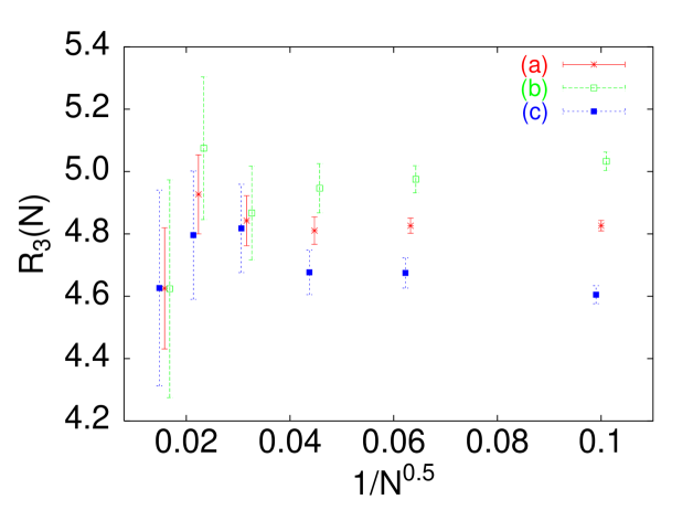
FIG. 1.: Estimates of $R_{3}(N)$ vs $1/N^{0.5}$ for three different cases: (a) $w_{1}=0.775$, $w_{2}=0.375$, (b) $w_{1}=0.775$, $w_{2}=0.505838$; (c) $w_{1}=0.375$, $w_{2}=0.505838$.

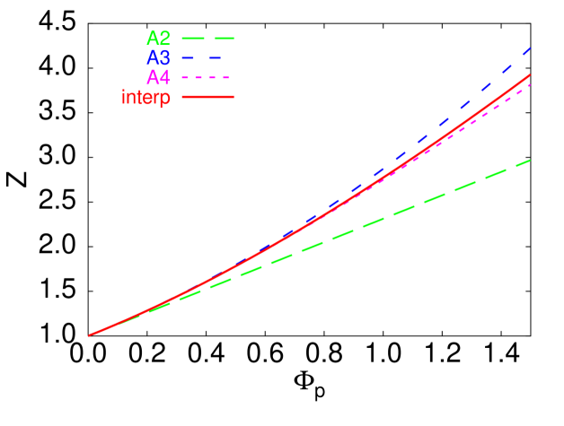
FIG. 2.: Compressibility factor $Z$ vs $\Phi_{p}$. We report four different approximations: (A2) it corresponds to Eq. (49) truncated to order $\Phi_{p}$; (A3) truncation to order $\Phi_{p}^{2}$; (A4) truncation to order $\Phi_{p}^{3}$; (interp) interpolation formula (53). In all cases $k_{\Phi}=0$.

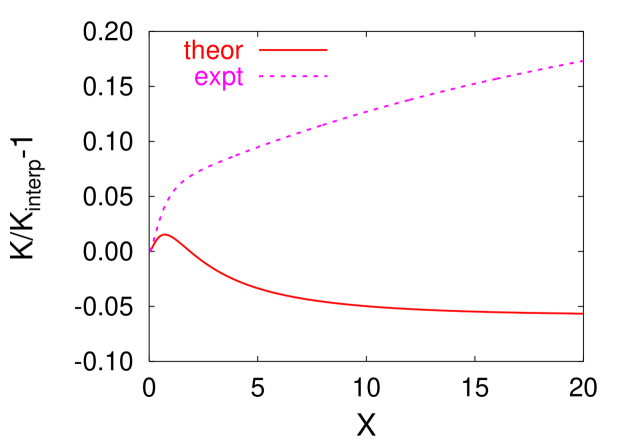
FIG. 3.: Comparison of the compressibility $K$ obtained by using the interpolation formula (53) ($K_{\rm interp}$) and two different approximations presented in Ref. [24]: one is based on one-loop field theory (“theor”), one is obtained by fitting different sets of data for polystyrene (“expt”).

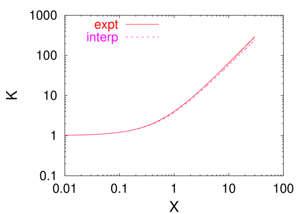
FIG. 4.: Comparison of the compressibility $K$ obtained by using the interpolation formula (53) (“interp”) and by fitting different sets of data for polystyrene (“expt”) (taken from Ref. [24]).

REFERENCES

• [1] P.G. de Gennes, Phys. Lett. 38A, 339 (1972).
• [2] P.G. de Gennes, Scaling Concepts in Polymer Physics (Cornell University Press, Ithaca, NY, 1979).
• [3] K.F. Freed, Renormalization Group Theory of Macromolecules (Wiley, New York, 1987).
• [4] L. Schäfer, Excluded Volume Effects in Polymer Solutions (Springer Verlag, Berlin, 1999).
• [5] At present the most accurate estimates of $\nu$ are $\nu=0.58758\pm 0.00007$ (Ref. [10]), $\nu=0.5874\pm 0.0002$ [T. Prellberg, J. Phys. A 34, L599 (2001)], $\nu=0.58765\pm 0.00020$ [H.-P. Hsu, W. Nadler, and P. Grassberger, Macromolecules 37, 4658 (2004)]. For an extensive list of results, see: A. Pelissetto and E. Vicari, Phys. Rept. 368, 549 (2002).
• [6] In experimental works the virial coefficients are usually defined from the expansion of $Z/M$ in terms of the ponderal concentration $\rho$, $Z/M=1/M+\sum_{n}B_{n+1}^{\rm expt}\rho^{n}$, where $M$ is the molar mass of the polymer. The coefficients $B_{n}^{\rm expt}$ are related to those we have defined by $B_{n}^{\rm expt}=N_{A}^{n-1}B_{n}M^{-n}$, where $N_{A}$ is the Avogadro number.
• [7] A. Pelissetto and J.-P. Hansen, J. Chem. Phys. 122, 134904 (2005).
• [8] B. Li, N. Madras, and A.D. Sokal, J. Stat. Phys. 80, 661 (1995).
• [9] B.G. Nickel, Macromolecules 24, 1358 (1991).
• [10] P. Belohorec and B.G. Nickel, “Accurate universal and two-parameter model results from a Monte-Carlo renormalization group study,” Guelph University report (1997), unpublished.
• [11] C. Domb and G.S. Joyce, J. Phys. C 5, 956 (1972).
• [12] J.-P. Hansen and I.R. McDonald, Theory of Simple Liquids, third ed. (Academic Press, New York, 2006).
• [13] M. Lal, Molec. Phys. 17, 57 (1969).
• [14] B. MacDonald, N. Jan, D.L. Hunter and M.O. Steinitz, J. Phys. A: Math. Gen. 18, 2627 (1985).
• [15] N. Madras and A.D. Sokal, J. Stat. Phys. 50, 109 (1988).
• [16] A.D. Sokal, in Monte Carlo and Molecular Dynamics Simulations in Polymer Science, edited by K. Binder (Oxford Univ. Press, Oxford, 1995).
• [17] T. Kennedy, J. Stat. Phys. 106, 407 (2002).
• [18] S. Caracciolo, G. Parisi, and A. Pelissetto, J. Stat. Phys. 77, 519 (1994).
• [19] In Ref. [7] the authors also report estimates of the contribution $I_{3}$ to the third virial coefficient. The contribution $T_{1}$ (that is small but not negligible) was not included and thus those results provide only an approximate estimate of the universal constant $A_{3}^{*}$. The contribution $T_{1}$ is also neglected in K. Shida, K. Ohno, Y. Kawazoe, and Y. Nakamura, J. Chem. Phys. 117, 9942 (2002), and in the expression reported in Ref. [8].
• [20] K. Shida, K. Ohno, M. Kimura, and Y. Kawazoe, Comput. Theor. Polymer Sc. 10, 281 (2000).
• [21] J. des Cloizeaux and I. Noda, Macromolecules 15, 1505 (1982).
• [22] J.F. Douglas and K.F. Freed, Macromolecules 18, 201 (1985).
• [23] In Sec. 17.3.2 of Ref. [4] field theory is used to obtain a prediction for the virial expansion. In terms of the variable $\hat{s}=4\pi cR_{g}^{3}/(3\times 1.169)$, $Z=1+1.433\hat{s}+1.065\hat{s}^{2}-0.648\hat{s}^{3}+\cdots$. This implies $Z=1+5.13cR_{g}^{3}+13.7(cR_{g}^{3})^{2}-30(cR_{g}^{3})^{3}+\cdots$. Note that also $A_{3}^{*}$ is considerably different from our result.
• [24] G. Merkle, W. Burchard, P. Lutz, K. F. Freed, and J. Gao, Macromolecules 26, 2736 (1993).
• [25] Eq. 17.52 of Ref. [4] gives the following expression for $Z$: $Z=1+1.314\Phi_{p}(H_{1}/H_{2})^{0.309}$, $H_{1}=1+2.15\Phi_{p}+1.00\Phi_{p}^{2}$, $H_{2}=1+0.51\Phi_{p}$. The variable $\hat{s}$ used in Ref. [4] is related to $\Phi_{p}$ by $\Phi_{p}=1.169\hat{s}$ (see Sec. 13.3.2). For $\Phi_{p}\to\infty$ it predicts $Z\approx 1.61\Phi_{p}^{1.309}$, that is slightly lower than the prediction $Z\approx 1.99\Phi_{p}^{1.309}$, reported in Sec. 17.4.1 of the same reference, indicating that the expected error on the parametrization should be of the order of 10%.
• [26] C.I. Addison, A.A. Louis, J. P. Hansen, J. Chem. Phys. 121, 612 (2004).
• [27] I. Noda, N. Kato, T. Kitano, and M. Nasagawa, Macromolecules 14, 668 (1981).
• [28] D.E. Knuth, The Art of Computer Programming, Vol. 2: Seminumerical Algorithms, Third Edition (Addison-Wesley, Reading, Massachusetts, 1997).
• [29] G. Parisi and F. Rapuano, Phys. Lett. B 157, 301 (1985).