Thermodynamics of spin systems on small-world hypergraphs

Abstract

We study the thermodynamic properties of spin systems on small-world hypergraphs, obtained by superimposing sparse Poisson random graphs with $p$-spin interactions onto a one-dimensional Ising chain with nearest-neighbor interactions. We use replica-symmetric transfer-matrix techniques to derive a set of fixed-point equations describing the relevant order parameters and free energy, and solve them employing population dynamics. In the special case where the number of connections per site is of the order of the system size we are able to solve the model analytically. In the more general case where the number of connections is finite we determine the static and dynamic ferromagnetic-paramagnetic transitions using population dynamics. The results are tested against Monte-Carlo simulations.

I Introduction

In recent years, a large amount of work has been devoted to the study of small-world networks, mainly numerical pekalski with emphasis e.g. on biophysical networks girvan -barabasi_nature or social networks newman and, to a lesser extent, analytically barratw ; reptrans . For recent reviews see e.g. albert-barabasi - bookbarabasi . By now, it has thus become apparent that small-world architectures can be found in many different circumstances, ranging from linguistic, epidemic and social networks to the world-wide-web.

Efficient modeling of real-world applications not only often requires a diluted random graph to describe the interaction network but, moreover, these interactions sometimes couple $k$-plets of agents. For instance, it has been found that the proteomic network of yeast forms a hypergraph with the proteins corresponding to vertices and the protein-complexes corresponding to hyperedges ramadan . Other large metabolic networks like the one of E. coli have also been found to possess a small-world structure and as most of the reactions of metabolism are multi-molecular they can be represented by hypergraphs wagner . Technical analysis of sparse hypergraphs is, however, involved even without superimposing small-world architectures.

A convenient way to describe the statistical physics of this type of systems is to consider diluted random graphs with $p$-spin interactions. In this context, a ferromagnetic model having $3$-spin interactions and finite connectivity has been considered recently in ferroglass . (See also barratz ; ricci ).

A complete description of a small-world system requires in addition local interactions. A simple example of the latter is the nearest-neighbor ferromagnetic Ising interaction. The inclusion of such local interactions can completely change the functioning and the dynamics of such systems. It was shown in reptrans , e.g., that this construction significantly enlarges the region in parameter space where ferromagnetism occurs. In particular, for any choice of the value of the average connectivity, however small, the ferromagnetic-paramagnetic transition occurs at a finite temperature. Furthermore, a jump in the entropy of metastable configurations has been found heylen exactly at the crossover between the small-world and the Poisson random graph structure due to the formation of disconnected clusters within the graph.

In this work we study the thermodynamic properties of such a small-world hypergraph, obtained by superimposing sparse Poisson random graphs with $p$-spin interactions onto a one-dimensional Ising chain with nearest-neighbor interactions. An analytic study of this model is non-trivial. The relevant disorder-averaged free energy and order parameters are calculated using replica-symmetric transfer-matrix techniques. A set of fixed-point equations for the order parameter functions is derived and solved numerically with the population dynamics algorithm mezardparisi . For $p=2$ we find back some of the results described in reptrans , 1infty ; kardar , for $p\geq 3$ the physics is different. In the limit where the number of long-range short-cuts are of the order of the system size for each site we get a mean-field model for which we are able to solve the order parameters in a completely analytic way, again using transfer matrices. First-order phase transitions from the ferromagnetic to the paramagnetic phase are found for all values of $p$, along with metastable (spinodal) transitions. Additionally, for $p=2$ a second-order phase transition and a coexistence region between the two phases are found.

Monte-Carlo simulations of the system employing Glauber dynamics allow us to find the dynamic (metastable) transition-lines. Very good agreement with the theory is found when the Ising chain interactions are ferromagnetic. When they are anti-ferromagnetic we find that the dynamics becomes very slow, indicating critical slowing down in this region. The rest of this paper is organized as follows. In Sec. II we define the small-world model. In Sec. III.1 we derive the saddle-point equations for the relevant order parameter function. Sec. III.2 discusses the transfer-matrix analysis in the replica symmetric approximation leading to a set of fixed-point equations involving the eigenvectors. Expressions for the free energy and the physical order parameters are given in Sec. III.3. There, we also discuss the continuous bifurcations from zero magnetization. Sec. IV gives the analytic solution of the fully connected version of the model. In Sec. V we numerically study the fixed-point equations and compare the results with simulations. Finally, Sec. VI contains the concluding remarks.

II The model

Consider a system of $N$ Ising spins $\mbox{\boldmath$\sigma$}=(\sigma_{1},\ldots,\sigma_{N})$, with $\sigma_{i}\in\{-1,1\}$, arranged on a one-dimensional chain ($\sigma_{N+1}=\sigma_{1})$. Two different couplings are assumed to be present in this system: first, nearest-neighbor interactions of uniform strength $J_{0}$ and, secondly, sparse long-range $p$-spin interactions of the form $c_{j_{1},\ldots,j_{p}}\sigma_{j_{1}}\ldots\sigma_{j_{p}}$, $\forall j_{\ell}\in\{1,2,\ldots,N\}$, of uniform strength $J$, which can be described by a hypergraph of degree $p$. An example of such a system for $p=3$ is shown in Fig. 1.

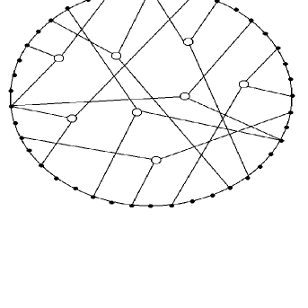
Figure 1: Schematic representation of a hypergraph of degree $3$ superimposed onto an Ising chain. Each black dot represents a spin, whereas each circle represents a hyperedge involving 3 spins

The couplings $c_{j_{1},\ldots,j_{p}}$ are independent identically distributed random variables, for $j_{1}<j_{2}<\ldots<j_{p}$, taken from the following distribution

$$P(c_{j_{1},\ldots,j_{p}}) = c\ \frac{(p-1)!}{N^{p-1}}\ \delta_{c_{j_{1},\ldots,j_{p}},1}$$ (1)

$$+\left(1-c\ \frac{(p-1)!}{N^{p-1}}\right)\ \delta_{c_{j_{1},\ldots,j_{p}},0}$$

The value $c_{j_{1},\ldots,j_{p}}=1$ indicates that the hyperedge formed by the $p$ spins $(\sigma_{j_{1}},\ldots,\sigma_{j_{p}})$ is present, whereas $c_{j_{1},\ldots,j_{p}}=0$ means that there is no such hyperedge present. The quantity $c$ indicates the total number of hyperedges a spin $\sigma$ is, on average, part of

$$\frac{1}{N}\sum_{i}\sum_{j_{1}<\ldots<j_{p-1}}c_{i,j_{1},\ldots,j_{p-1}}=c$$ (2)

In the small-world context one takes $c$ to be a small number of order ${\cal O}(1)$ while $c/N\rightarrow 0$.

We assume that the couplings are symmetric such that for any permutation $\pi$ in $\mathcal{S}_{p}$ (the symmetric group of $p$ elements):

$$c_{j_{1},\ldots,j_{p}}=c_{j_{\pi(1)},\ldots,j_{\pi(p)}}$$ (3)

Furthermore, we exclude self-interactions and hyperedges of reduced degree by stating that

$$\forall k\neq l\in\{1,\ldots,p\}:j_{k}=j_{l}\Rightarrow c_{j_{1},\ldots,j_{p}}=0$$ (4)

meaning that the hyperedge does not exist when any two indices are equal.

At thermal equilibrium, such a system can be described by the Hamiltonian

$$H(\mbox{\boldmath$\sigma$})=-\sum_{i}\sigma_{i}h_{i}(\mbox{\boldmath$\sigma$})$$ (5)

where the local field consists of a hypergraph part and a chain part

$$h_{i}(\mbox{\boldmath$\sigma$}) = \frac{J}{cp}\sum_{j_{1}<\ldots<j_{p-1}}c_{i,j_{1},\ldots,j_{p-1}}\sigma_{j_{1}}\ldots\sigma_{j_{p-1}}$$ (6)

$$+\frac{J_{0}}{2}(\sigma_{i-1}+\sigma_{i+1})$$

We want to study the thermodynamic properties of this network structure which follow from the free energy per site

$$f=-\lim_{N\to\infty}\frac{1}{\beta N}\log\sum_{\mbox{\boldmath$\sigma$}}e^{-\beta H(\mbox{\boldmath$\sigma$})}$$ (7)

where $\beta=1/T$ corresponds to the inverse bath temperature.

III Replicated transfer-matrix analysis

III.1 Saddle-point equations

We start from the free energy per spin written down in the replica approach MPV

$$-\beta f(\beta) = \lim_{N\to\infty}\,\,\lim_{n\to 0}\frac{1}{Nn}\log\langle Z^{n}\rangle_{\mbox{\boldmath$c$}}$$ (8)

$$\langle Z^{n}\rangle_{\mbox{\boldmath$c$}} = \sum_{\mbox{\boldmath$\sigma$}^{1},\ldots,\mbox{\boldmath$\sigma$}^{n}}\left\langle\exp\left(-\beta\sum_{\alpha}H(\mbox{\boldmath$\sigma$}^{\alpha})\right)\right\rangle_{\mbox{\boldmath$c$}}$$ (9)

with $\alpha=1,\ldots,n$ the replica index and the average taken over all possible graphs $c$ according to the distribution (1), so that we obtain

$$\langle Z^{n}\rangle_{\mbox{\boldmath$c$}}=\sum_{\mbox{\boldmath$\sigma$}^{1},\ldots,\mbox{\boldmath$\sigma$}^{n}}\exp\left(\beta J_{0}\sum_{i,\alpha}\sigma_{i}^{\alpha}\sigma_{i+1}^{\alpha}\right)$$

$$\times \prod_{j_{1}<\ldots<j_{p}}\left\langle\exp\left(\frac{\beta J}{c}\sum_{\alpha}c_{j_{1},\ldots,j_{p}}\sigma_{j_{1}}^{\alpha}\ldots\sigma_{j_{p}}^{\alpha}\right)\right\rangle_{c_{j_{1},\ldots,j_{p}}}$$

$$= \sum_{\mbox{\boldmath$\sigma$}^{1},\ldots,\mbox{\boldmath$\sigma$}^{n}}\exp\left(\beta J_{0}\sum_{i,\alpha}\sigma_{i}^{\alpha}\sigma_{i+1}^{\alpha}\right)$$

$$\times \exp\left(\frac{c\ (p-1)!}{N^{p-1}}\sum_{j_{1}<\ldots<j_{p}}\left(e^{\frac{\beta J}{c}\sum_{\alpha}\sigma_{j_{1}}^{\alpha}\ldots\sigma_{j_{p}}^{\alpha}}-1\right)\right)$$ (11)

where we have used the fact that $N\rightarrow\infty$ to contract the average over $c_{j_{1},\ldots,j_{p}}$ into an exponential.

The next step is to insert unities $1=\sum_{\mbox{\boldmath$\sigma$}}\delta_{\mbox{\boldmath$\sigma$},\mbox{\boldmath$\sigma$}_{i}}$ and $1=\sum_{\mbox{\boldmath$\tau$}}\delta_{\mbox{\boldmath$\tau$},\mbox{\boldmath$\sigma$}_{j}}$ where $\mbox{\boldmath$\sigma$},\mbox{\boldmath$\tau$}$ are auxiliary vectors in replica space to arrive at

$$\langle Z^{n}\rangle_{\mbox{\boldmath$c$}}=\sum_{\mbox{\boldmath$\sigma$}^{1},\ldots,\mbox{\boldmath$\sigma$}^{n}}\exp\left(\beta J_{0}\sum_{i,\alpha}\sigma_{i}^{\alpha}\sigma_{i+1}^{\alpha}\right)$$ (12)

$$\times \exp\left(\frac{c}{pN^{p-1}}\sum_{\mbox{\boldmath$\tau$}_{1}\ldots\mbox{\boldmath$\tau$}_{p}}\prod_{k=1}^{p}\sum_{j_{k}}\delta_{\mbox{\boldmath$\tau$}_{k},\mbox{\boldmath$\sigma$}_{j_{k}}}\right.$$

$$\times \left.\left(e^{\frac{\beta J}{c}\sum_{\alpha}\tau_{1}^{\alpha}\ldots\tau_{p}^{\alpha}}-1\right)\right.\Bigg{)}$$

In this way we have effectively introduced an order function

$$F(\mbox{\boldmath$\tau$})=\frac{1}{N}\sum_{i}\delta_{\mbox{\boldmath$\tau$},\mbox{\boldmath$\sigma$}_{i}}$$ (13)

that can be inserted in (12) in the usual way

$$1=\int\prod_{\mbox{\boldmath$\tau$}}dF(\mbox{\boldmath$\tau$})d\hat{F}(\mbox{\boldmath$\tau$})\ e^{i\hat{F}(\mbox{\boldmath$\tau$})\left(F(\mbox{\boldmath$\tau$})-\frac{1}{N}\sum_{i}\delta_{\mbox{\boldmath$\tau$},\mbox{\boldmath$\sigma$}_{i}}\right)}$$ (14)

to obtain

$$\langle Z^{n}\rangle_{\mbox{\boldmath$c$}}\sim\int\left[\prod_{\mbox{\boldmath$\tau$}}dF(\mbox{\boldmath$\tau$})d\hat{F}(\mbox{\boldmath$\tau$})\right]\exp\left[iN\sum_{\mbox{\boldmath$\tau$}}\hat{F}(\mbox{\boldmath$\tau$})F(\mbox{\boldmath$\tau$})\right]$$ (15)

$$\times \exp\left(\frac{cN}{p}\sum_{\mbox{\boldmath$\tau$}_{1}\ldots\mbox{\boldmath$\tau$}_{p}}\prod_{k=1}^{p}F(\mbox{\boldmath$\tau$}_{k})\left(e^{\frac{\beta J}{c}\sum_{\alpha}\tau_{1}^{\alpha}\ldots\tau_{p}^{\alpha}}-1\right)\right)$$

$$\times \sum_{\mbox{\boldmath$\sigma$}^{1},\ldots,\mbox{\boldmath$\sigma$}^{n}}\exp\left(\beta J_{0}\sum_{i,\alpha}\sigma_{i}^{\alpha}\sigma_{i+1}^{\alpha}-i\sum_{i}\hat{F}(\mbox{\boldmath$\sigma$}_{i})\right)$$

We can then apply the saddle-point method resulting in

$$\log\left(\langle Z^{n}\rangle_{\mbox{\boldmath$c$}}\right)=\underset{F,\hat{F}}{\rm Extr}\left[i\sum_{\mbox{\boldmath$\tau$}}\hat{F}(\mbox{\boldmath$\tau$})F(\mbox{\boldmath$\tau$})\right.$$ (16)

$$+ \left.\frac{c}{p}\sum_{\mbox{\boldmath$\tau$}_{1}\ldots\mbox{\boldmath$\tau$}_{p}}\prod_{k=1}^{p}F(\mbox{\boldmath$\tau$}_{k})\left(e^{\frac{\beta J}{c}\sum_{\alpha}\tau_{1}^{\alpha}\ldots\tau_{p}^{\alpha}}-1\right)\right.$$

$$+ \left.\frac{1}{N}\log\left(\sum_{\mbox{\boldmath$\sigma$}^{1},\ldots,\mbox{\boldmath$\sigma$}^{n}}e^{\beta J_{0}\sum_{i\alpha}\sigma_{i}^{\alpha}\sigma_{i+1}^{\alpha}-i\sum_{i}\hat{F}(\mbox{\boldmath$\sigma$}_{i})}\right)\right]$$

Derivation with respect to $F(\mbox{\boldmath$\psi$})$ and $\hat{F}(\mbox{\boldmath$\psi$})$ results in the following self-consistent equation for the density $F(\psi)$:

$$F(\mbox{\boldmath$\psi$})=\frac{\sum_{\mbox{\boldmath$\sigma$}_{1}\ldots\mbox{\boldmath$\sigma$}_{N}}\left[\frac{1}{N}\sum_{i}\delta_{\mbox{\boldmath$\sigma$}_{i},\mbox{\boldmath$\psi$}}\right]\exp\left(\beta J_{0}\sum_{j\alpha}\sigma_{j}^{\alpha}\sigma_{j+1}^{\alpha}+c\sum_{j}\sum_{\mbox{\boldmath$\tau$}_{1}\ldots\mbox{\boldmath$\tau$}_{p-1}}\prod_{k=1}^{p-1}F(\mbox{\boldmath$\tau$}_{k})\left(e^{\frac{\beta J}{c}\sum_{\alpha}\tau_{1}^{\alpha}\ldots\tau_{p-1}^{\alpha}\sigma_{j}^{\alpha}}-1\right)\right)}{\sum_{\mbox{\boldmath$\sigma$}^{1}\ldots\mbox{\boldmath$\sigma$}^{n}}\exp\left(\beta J_{0}\sum_{j\alpha}\sigma_{j}^{\alpha}\sigma_{j+1}^{\alpha}+c\sum_{j}\sum_{\mbox{\boldmath$\tau$}_{1}\ldots\mbox{\boldmath$\tau$}_{p-1}}\prod_{k=1}^{p-1}F(\mbox{\boldmath$\tau$}_{k})\left(e^{\frac{\beta J}{c}\sum_{\alpha}\tau_{1}^{\alpha}\ldots\tau_{p-1}^{\alpha}\sigma_{j}^{\alpha}}-1\right)\right)}$$ (17)

In the absence of short-range bonds, i.e. $J_{0}=0$, this expression factorizes over sites and can be reduced considerably. In our case, however, this is not possible and in order to perform the spin summations we are now required to construct transfer matrices.

III.2 Transfer-matrix analysis

Defining the following $2^{n}\times 2^{n}$ matrix

$$T_{\mbox{\boldmath$\sigma$},\mbox{\boldmath$\tau$}}[F]=\exp\left(\beta J_{0}\sum_{\alpha}\sigma^{\alpha}\tau^{\alpha}\right)$$

$$\times \exp\left(c\sum_{\mbox{\boldmath$\tau$}_{1}\ldots\mbox{\boldmath$\tau$}_{p-1}}\prod_{k=1}^{p-1}F(\mbox{\boldmath$\tau$}_{k})\left(e^{\frac{\beta J}{c}\sum_{\alpha}\tau_{1}^{\alpha}\ldots\tau_{p-1}^{\alpha}\sigma^{\alpha}}-1\right)\right)$$

Eq. (17) reads

$$F(\mbox{\boldmath$\psi$})=$$

$$\frac{\sum_{j}\sum_{\mbox{\boldmath$\sigma$}_{1}\mbox{\boldmath$\sigma$}_{j}}\left(T^{j-1}[F]\right)_{\mbox{\boldmath$\sigma$}_{1}\mbox{\boldmath$\sigma$}_{j}}\delta_{\mbox{\boldmath$\sigma$}_{j},\mbox{\boldmath$\psi$}}\left(T^{N-j+1}[F]\right)_{\mbox{\boldmath$\sigma$}_{j}\mbox{\boldmath$\sigma$}_{1}}}{N\ \textnormal{tr}\>(T^{N}[F])}$$

We insert unity $1=\sum_{\mbox{\boldmath$\tau$}}\delta_{\mbox{\boldmath$\sigma$}_{j},\mbox{\boldmath$\tau$}}$ and introduce the matrix $Q_{\mbox{\boldmath$\sigma$}_{j}\mbox{\boldmath$\tau$}}(\mbox{\boldmath$\psi$})=\delta_{\mbox{\boldmath$\sigma$}_{j},\mbox{\boldmath$\psi$}}\delta_{\mbox{\boldmath$\sigma$}_{j},\mbox{\boldmath$\tau$}}$ to obtain after some algebra

$$F(\mbox{\boldmath$\psi$})=\frac{\textnormal{tr}\>(T^{N}[F]Q(\mbox{\boldmath$\psi$}))}{\textnormal{tr}\>(T^{N}[F])}$$ (20)

To proceed with the evaluation of the traces in (20) we remark that in the thermodynamic limit $N\rightarrow\infty$ only $\lambda_{0}$, the largest eigenvalue of $T[F]$ will contribute. Defining

$$\sum_{\mbox{\boldmath$\tau$}}T_{\mbox{\boldmath$\sigma$},\mbox{\boldmath$\tau$}}[F]u(\mbox{\boldmath$\tau$}) = \lambda_{0}u(\mbox{\boldmath$\sigma$})$$ (21)

$$\sum_{\mbox{\boldmath$\sigma$}}v(\mbox{\boldmath$\sigma$})T_{\mbox{\boldmath$\sigma$},\mbox{\boldmath$\tau$}}[F] = \lambda_{0}v(\mbox{\boldmath$\tau$})$$ (22)

we have that

$$T^{N}_{\mbox{\boldmath$\sigma$},\mbox{\boldmath$\tau$}}[F]\approx\lambda_{0}^{N}u(\mbox{\boldmath$\sigma$})v(\mbox{\boldmath$\tau$})$$ (23)

and consequently

$$F(\mbox{\boldmath$\psi$})=\frac{u(\mbox{\boldmath$\psi$})v(\mbox{\boldmath$\psi$})}{\sum_{\mbox{\boldmath$\sigma$}}u(\mbox{\boldmath$\sigma$})v(\mbox{\boldmath$\sigma$})}$$ (24)

So, in order to find a solution for $F(\mbox{\boldmath$\psi$})$ we need to solve the equations (21), (22) and (24).

At this point we invoke replica symmetry (RS) by assuming that $\forall\pi\in\mathcal{S}_{n}:F(\mbox{\boldmath$\psi$})=F(\pi(\mbox{\boldmath$\psi$})).$ One way to fulfil this is to write $F(\mbox{\boldmath$\psi$})$ as follows mezardparisi

$$F(\mbox{\boldmath$\psi$})=\int dh\>W(h)\prod_{\alpha=1}^{n}\frac{e^{\beta h\psi^{\alpha}}}{2\cosh(\beta h)}$$ (25)

The density $W(h)$ is normalised. We also assume the left and right eigenvectors to be replica symmetric

$$u(\mbox{\boldmath$\psi$}) = \int dx\>\phi(x)\prod_{\alpha=1}^{n}e^{\beta x\psi^{\alpha}}$$ (26)

$$v(\mbox{\boldmath$\psi$}) = \int dy\>\chi(y)\prod_{\alpha=1}^{n}e^{\beta y\psi^{\alpha}}$$ (27)

This allows us to write down self-consistent equations for $\phi(x)$ and $\chi(x)$. We insert Eqs. (25) and (26) into the l.h.s of Eq. (21) and obtain after some algebra (see the Appendix for more details) the following closed equation for $n\rightarrow 0$

$$\lambda_{0}\phi(x^{\prime})=\sum_{\mu=0}^{\infty}\left\{\frac{e^{-c}c^{\mu}}{\mu!}\left[\prod_{\nu=1}^{\mu}\prod_{k=1}^{p-1}\!\int\!dh_{k}^{\nu}\>W(h_{k}^{\nu})\right]\!\int\!dx\>\phi(x)\right.$$ (28)

$$\times\left.\delta\left[x^{\prime}-\frac{1}{\beta}\left[\sum_{\nu=1}^{\mu}{\rm{atanh}}\left(\tanh(\frac{\beta J}{c})\prod_{k=1}^{p-1}\tanh(\beta h_{k}^{\nu})\right)\right.\right.\right.$$

$$\left.\left.+{\rm{atanh}}\left(\tanh(\beta x)\tanh(\beta J_{0})\Bigg{)}\right]\right]\right\}$$

In a similar way we derive a self-consistent equation for $\chi(x)$ by inserting (25) and (27) into the l.h.s. of Eq. (22)

$$\lambda_{0}\chi(x^{\prime}) = \sum_{\mu=0}^{\infty}\left(\frac{e^{-c}c^{\mu}}{\mu!}\left[\prod_{\nu=1}^{\mu}\prod_{k=1}^{p-1}\int dh_{k}^{\nu}\>W(h_{k}^{\nu})\right]\right.$$ (29)

$$\left.\int dx\>\chi(x)\delta\left[x^{\prime}-\frac{1}{\beta}{\rm{atanh}}\left[\tanh(\beta J_{0})\tanh\left(\beta x+\sum_{\nu=1}^{\mu}{\rm{atanh}}(\tanh(\frac{\beta J}{c})\prod_{k}\tanh(\beta h_{k}^{\nu}))\right)\right]\right]\right\}$$

At this point we choose the $\phi(x)$ and $\chi(x)$ to be normalised. We remark that in the limit $c\rightarrow 0$, $J\rightarrow 0$ or $p\rightarrow\infty$ equations (28) and (29) reduce correctly to those of a one-dimensional Ising chain.

Next, to find the self-consistent equation for $W(h)$ we start from Eq. (24) and fill in the RS-assumptions (26) and (27). Requiring that the resulting expression takes in the limit $n\rightarrow 0$ the form of Eq. (25) we obtain

$$W(h)=\int dx\>dy\>\phi(x)\chi(y)\delta(h-x-y)$$ (30)

Finally, in order to calculate the free energy per spin we need to determine the largest eigenvalue $\lambda_{0}$ in the limit $n\rightarrow 0$. We start from Eq. (21), insert Eqs. (25) and (26) to obtain

$$\lambda_{0}=1+n\sum_{\mu=0}^{\infty}\frac{e^{-c}c^{\mu}}{\mu!}\prod_{\nu=1}^{\mu}\prod_{k=1}^{p-1}\int dh_{k}^{\nu}\>W(h_{k}^{\nu})\int dx\>\phi(x)$$ (31)

$$\times\left(\frac{1}{2}\sum_{s}\left(\log\left(G^{R}_{s}(x,\{h_{k}^{\nu}\})\right)\right)-\log(2\cosh((\beta h_{k}^{\nu})))\right)$$

$$+{\cal O}(n^{2})$$

with

$$G^{R}_{s}(x,\{h_{k}^{\nu}\})=\left(\sum_{\gamma=\pm 1}e^{\beta\gamma(x+J_{0}s)}\right)$$ (32)

$$\times \prod_{\nu=1}^{\mu}\sum_{\gamma_{1}\ldots\gamma_{p-1}}e^{\beta\sum_{k=1}^{p-1}h_{k}^{\nu}\gamma_{k}+\frac{\beta J}{c}\gamma_{1}\ldots\gamma_{p-1}s}$$

So $\lambda_{0}=1$ in the limit $n\rightarrow 0$.

III.3 Thermodynamics

We can now evaluate the free energy per spin. Starting from (8) and (16) we arrive at

$$-\beta f(\beta) = \frac{c(1-p)}{p}\left[\prod_{k=1}^{p}\int dh_{k}\>W(h_{k})\right]\left[\log\left(\sum_{\tau_{1}\ldots\tau_{p}}e^{\beta\sum_{k}h_{k}\tau_{k}+\frac{\beta J}{c}\tau_{1}\ldots\tau_{p}}\right)-\log\left(\sum_{\tau_{1}\ldots\tau_{p}}e^{\beta\sum_{k}h_{k}\tau_{k}}\right)\right]$$ (33)

$$+\sum_{\mu=0}^{\infty}\frac{e^{-c}c^{\mu}}{\mu!}\prod_{\nu=1}^{\mu}\prod_{k=1}^{p-1}\int dh_{k}^{\nu}\>W(h_{k}^{\nu})\int dx\>\phi(x)\left(\frac{1}{2}\sum_{s}\left(\log\left(G^{R}_{s}(x,\{h_{k}^{\nu}\})\right)\right)-\log(2\cosh((\beta h_{k}^{\nu})))\right)$$

which is the final result. As the elements of the adjacency matrix $c_{i_{1},\ldots,i_{p}}$ have been taken i.i.d. one would expect the degrees at each site to be Poisson distributed. Indeed, we see that this has come out naturally from the analysis and we can associate the average over the Poisson probabilities in (28,29,33) as an average over degrees.

The order parameters of the system under study are the average magnetization which reads, recalling Eq. (25)

$$m_{\alpha} = \left\langle\frac{1}{N}\sum_{i}\sigma_{i}^{\alpha}\right\rangle_{\mbox{\boldmath$c$}}$$ (34)

$$\overset{\text{RS}}{=} \int dh\>W(h)\tanh(\beta h)$$ (35)

and the Edwards-Anderson parameter function

$$q_{\alpha\beta} = \left\langle\left(\frac{1}{N}\sum_{i}\sigma_{i}^{\alpha}\sigma_{i}^{\beta}\right)\right\rangle_{\mbox{\boldmath$c$}}\,\,\,,\qquad\alpha\neq\beta$$ (36)

$$\overset{\text{RS}}{=} \int dh\>W(h)\tanh^{2}(\beta h)$$ (37)

We remark that due to the RS assumption $m_{\alpha}=m$ for $\forall\alpha$, $q_{\alpha\beta}=q$ for $\forall\alpha\neq\beta$, and $q_{\alpha\alpha}=1$.

Next, in order to obtain the phase diagram we have to study the solutions of the self-consistent equations (28), (29) and (30). It is easily seen that the field-distributions $\phi(x)=\chi(x)=W(x)=\delta(x)$ are a solution of these equations, corresponding to the paramagnetic phase according to Eq. (35). For this solution the free energy per spin (33) reduces to

$$-\beta f_{\text{para}}(\beta) = \frac{c}{p}\log\cosh\left(\frac{\beta J}{c}\right)$$ (38)

$$+\log\cosh\left(\beta J_{0}\right)+\log(2)$$

For high temperatures, this is the only solution present. Following a standard procedure in finite-connectivity theory (see, e.g. reptrans ) we discuss continuous bifurcations away from this solution in order to find second-order phase transitions. Since we are dealing with field-distributions this means that the fields will be narrowly distributed around zero so that we can expand the equations (35) and (37), using equation (30). In order to quantify the difference with the deltapeak-solution we assume $\int dh\>h^{k}\phi(h)={\cal O}(\epsilon^{k})$ and $\int dh\>h^{k}\chi(h)={\cal O}(\epsilon^{k})$ with $|\epsilon|\ll 1$ such that

$$m = \beta\int dx\>\phi(x)x+\beta\int dy\>\chi(y)y+{\cal O}(\epsilon^{3})$$ (39)

$$q = \beta^{2}\int dx\>dy\>\phi(x)\chi(y)(x+y)^{2}+{\cal O}(\epsilon^{3})$$ (40)

In order to find the transition towards non-zero magnetization we look for bifurcations where the first moments become of order $\epsilon$. Introducing $\overline{x}=\int dx\>x\>\phi(x)$ and $\overline{y}=\int dy\>y\>\chi(y)$, and recalling Eqs. (28) and (29) we find the following set of self-consistent equations

$$\overline{x} = \overline{x}\tanh(\beta J_{0})+c\tanh(\frac{\beta J}{c})(\overline{x}+\overline{y})^{p-1}\beta^{p-2}\qquad$$ (41)

$$\overline{y} = \overline{y}\tanh(\beta J_{0})$$ (42)

$$+c\tanh(\beta J_{0})\tanh(\frac{\beta J}{c})(\overline{x}+\overline{y})^{p-1}\beta^{p-2}$$

For $p>2$ the second terms in the r.h.s. of these equations are of a higher order in $\epsilon$ and, hence, no second-order bifurcations to a ferromagnetic phase are found. For $p=2$ these equations do lead to a second-order bifurcation at

$$1=c\tanh(\frac{\beta J}{c})\exp(2\beta J_{0})$$ (43)

in agreement with reptrans .

Analogously, we can look for bifurcations to a spin-glass transition by expanding the second-order moments, assuming that $\overline{x}=\overline{y}=0$. Introducing $\overline{x^{2}}=\int dx\>x^{2}\>\phi(x)$ and $\overline{y^{2}}=\int dy\>y^{2}\>\chi(y)$ we get

$$\overline{x^{2}} = \overline{x^{2}}\tanh^{2}(\beta J_{0})$$ (44)

$$+c\tanh^{2}(\frac{\beta J}{c})\overline{(x+y)^{2(p-1)}}\beta^{p-2}$$

$$\overline{y^{2}} = \overline{y^{2}}\tanh^{2}(\beta J_{0})$$

$$+c\tanh^{2}(\beta J_{0})\tanh^{2}(\frac{\beta J}{c})\overline{(x+y)^{2(p-1)}}\beta^{p-2}$$

Again, from this we can deduce that there is no second-order spin-glass transition for $p>2$ but for $p=2$ a continuous bifurcation to $q>0,m=0$ occurs at

$$1=c\tanh^{2}(\frac{\beta J}{c})\cosh(2\beta J_{0})$$ (46)

The $p=2$ results are in agreement with those of reptrans , where it is also argued that for $J,J_{0}\geq 0$ the second-order paramagnetic to spin-glass instability cannot occur as it will always be preceded by the ferromagnetic one when lowering the temperature. From simulation experiments we find some evidence for glassy behavior at lower temperatures for all $p$, especially for $\beta J_{0}\leq 0$, as will be shortly discussed in Section V. There we also study first-order transitions by employing the transfer-matrix analysis developed in Sec. III.1,III.2 together with population dynamics.

IV The $1+\infty$ dimensional model

A limiting case of the previous results is a one-dimensional Ising chain superimposed on a fully connected hypergraph. This model gets a mean-field character and can be solved analytically by using the transfer-matrix approach. In the sequel we denote this model by the $1+\infty$ dimensional model.

In order to have a multispin interaction between every multiplet of $p$ spins we must take $c=N^{p-1}/(p-1)!$ (See e.g. equation (1)). Recalling the Hamiltonian (5) and the local field (6) this leads to the following free energy per spin

$$-\beta f = \lim_{N\rightarrow\infty}\frac{1}{N}\log\left(\underset{\mbox{\boldmath$\sigma$}}{\textnormal{Tr}\>}\exp\left(\frac{\beta J}{pN^{p-1}}\sum_{j_{1}}\ldots\sum_{j_{p}}\sigma_{j_{1}}\ldots\sigma_{j_{p}}+\beta J_{0}\sum_{i}\sigma_{i}\sigma_{i+1}\right)\right)$$ (47)

$$= \lim_{N\rightarrow\infty}\frac{1}{N}\log\left(\underset{\mbox{\boldmath$\sigma$}}{\textnormal{Tr}\>}\int dmd\hat{m}\exp\left(i\hat{m}(m-\frac{1}{N}\sum_{i}\sigma_{i})\right)\exp\left(\frac{\beta JN}{p}m^{p}+\beta J_{0}\sum_{i}\sigma_{i}\sigma_{i+1}\right)\right)$$ (48)

$$= \lim_{N\rightarrow\infty}\frac{1}{N}\log\left(\int dmd\hat{m}\exp\left(iN\hat{m}m+\frac{\beta JN}{p}m^{p}\right)\textnormal{Tr}\>\left[T^{N}\right]\right).$$ (49)

Here $T$ is the transfer-matrix

$$T=\left(\begin{array}[]{cc}e^{-i\hat{m}+\beta J_{0}}&e^{-i\hat{m}-\beta J_{0}}\\ e^{i\hat{m}-\beta J_{0}}&e^{i\hat{m}+\beta J_{0}}\end{array}\right)$$ (50)

The eigenvalues $\lambda$ of this matrix are

$$\lambda_{\pm}(\hat{m}) = e^{\beta J_{0}}\cosh(i\hat{m})$$ (51)

$$\pm\left(e^{2\beta J_{0}}\cosh^{2}(i\hat{m})-2\sinh(2\beta J_{0})\right)^{\frac{1}{2}}$$

Using the fact that for $\to\infty$ $\textnormal{Tr}\>\left[T^{N}\right]=\lambda_{+}^{N}+\lambda_{-}^{N}\approx\lambda_{+}^{N}$ we write equation (49) as

$$-\beta f = \lim_{N\rightarrow\infty}\frac{1}{N}\log\left(\int dmd\hat{m}\right.$$

$$\times\left.\exp\left(iN\hat{m}m+\frac{\beta JN}{p}m^{p}+N\log(i\lambda_{+}\hat{m})\right)\right)$$

In the limit $N\rightarrow\infty$, the fixed-point equation minimizing the free energy per spin is given by

$$m=G(m),\hskip 5.69054ptG(m)\equiv\frac{\sinh(\beta Jm^{p-1})}{\sqrt{\sinh^{2}(\beta Jm^{p-1})+e^{-4\beta J_{0}}}}$$ (53)

We remark that this equation reduces to the one presented in 1infty for $p=2$.

To find the phase diagram of this system we perform a bifurcation analysis. It is easy to see that $m=0$, which describes the paramagnetic phase, always satisfies Eq. (53) for any temperature. To find phase transitions away from the paramagnetic solution, we must find the critical parameter values for which the pair of equations $m=G(m)$ and $1=G^{\prime}(m)$ has new $m\neq 0$ solutions. These solutions can be created from $m=0$ (continuous bifurcation) or away from $m=0$ (discontinuous ones).

With these considerations we immediately observe that there are no solutions for $p>2$, but for $p=2$ we find the solution

$$\beta J=e^{-2\beta J_{0}}$$ (54)

To look for first-order transitions we have to find solutions to $m=G(m)$ and $1=G^{\prime}(m)$ at $m\neq 0$. In this model this can be done analytically by introducing the auxiliary variable

$$x=\beta Jm^{p-1},\qquad x\in[-\infty,\infty]/\{0\}$$ (55)

leading to the following two equations describing the transition line, parametrized by $x$:

$$\beta J_{0}(x) = -\frac{1}{4}\log\left(\frac{\tanh(x)\sinh^{2}(x)}{x(p-1)-\tanh(x)}\right)$$ (56)

$$\beta J(x) = {x}\left(\frac{x(p-1)}{x(p-1)-\tanh(x)}\right)^{\frac{1}{2}(p-1)}$$ (57)

We remark that in the limit $\beta J\to\infty$, the slope of $\beta J/\beta J_{0}$ approaches $-2$ and, hence, is $p$-independent.

For any non-zero $x$ we can now find a pair $\beta J$ and $\beta J_{0}$ at which a first order phase transition occurs. The value of the magnetization $m$ at that point is given by equation (55). These phase transition lines are plotted in Fig. 2 for several values of the degree $p$.

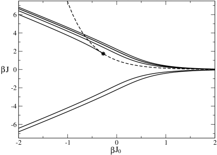
Figure 2: Phase diagram for the $1+\infty$ dimensional model in the $\beta J-\beta J_{0}$ plane for different $p$. The solid lines indicate first-order transitions: for $\beta J>0$, $p=2,3,4,5$ from bottom to top, and for $\beta J<0$, $p=3,5$ from top to bottom. The dashed line is the second-order transition line for $p=2$. The star indicates the tri-critical point for $p=2$.

We see that no transitions occur for even $p$ and $\beta J<0$. Furthermore, we remark the $\beta J$ symmetry for odd $p$, due to the symmetry properties of the Hamiltonian (5) and (6) under the change of sign $\mbox{\boldmath$\sigma$}\rightarrow-\mbox{\boldmath$\sigma$}$. The ferromagnetic phase is situated to the right of the transition lines, so for odd $p$ the paramagnetic phase is in between the symmetrical solid lines, for $p$ even it lies below the corresponding solid line. For increasing $p$, the ferromagnetic region decreases. For the special case of $p=2$ the paramagnetic and ferromagnetic phase coexist between the first and second-order transition lines with as tri-critical point $\beta J=\sqrt{3}\approx 1.732,\,\,\beta J_{0}=-\log(3)/4\approx-0.275$. The latter results are in agreement with the results of 1infty and with those of kardar in the case of one dimension. This analysis serves as a limiting case of our small-world model for increasingly larger values of the mean connectivity per site $c$.

V Results for finite $c$.

The main equations describing the thermodynamics of the small-world hypergraph for finite $c$ are Eqs. (28), (29) and (30). To solve these equations we use the population dynamics algorithm to generate field distributions together with Monte Carlo integration over the generated populations in order to obtain the physical parameters. The important parameters of this algorithm are the size of the populations and the number of iterations. The size of the populations has to be big enough to get clearly outlined distributions keeping in mind, however, that the computational time required for the algorithm to converge is linear in this parameter. In most cases we find that populations of 10000 fields give accurate results. The number of iterations per spin depends strongly on the physical parameters. It turns out that most of the time about 1000 iterations results in a reasonable accuracy. To calculate the ferromagnetic free energy it proves useful to average over several (e.g. 100) runs with different initial conditions.

From the $1+\infty$ dimensional model solved analytically in Section IV we learned already that the physics for $p=2$ versus the one for $p\geq 3$ might be very different. As a benchmark test for our derivations we have reproduced some of the results for $p=2$ found in reptrans ; kardar . We do not repeat them here but concentrate on $p\geq 3$ in the sequel.

Starting from the paramagnetic phase and lowering the temperature, ferromagnetic solutions will start to appear, indicating a dynamical transition which appears to be first order. However, to check which of these solutions is thermodynamically stable, we need to calculate the free energy of both the $m=0$ and $m\neq 0$ solutions. The former is given by (38), and the latter can be calculated numerically from (33). This leads to two special temperatures: the temperature where the first $m\neq 0$ solutions start to appear, also known as the spinodal point, dynamical transition or metastable transition, and the temperature where the ferromagnetic free energy becomes lower than the paramagnetic free energy, indicating the thermodynamic phase transition.

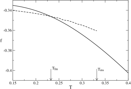
Figure 3: The free energy per spin as a function of temperature for $J=1$, $J_{0}=0$, $c=3$ and $p=3$. The dashed line indicates the free energy of the $m\neq 0$ state, while the solid line indicates the paramagnetic free energy. The thermodynamic phase transition occurs at the crossing of the two lines, whereas the spinodal point is the highest temperature for which an $m\neq 0$ solution is possible.

First, we calculate for general $p$ the critical temperatures at which these transitions occur. They are plotted for the the cases $p=3,4$ for the model without chain contribution ($J_{0}=0$) in Fig. 4 , and with chain contribution ($J_{0}=0.1$) in Fig. 5. Above the thermodynamic transition lines ($T_{fm}$) we find the paramagnetic phase, below the ferromagnetic phase. Metastable ferromagnetic states can be found up until the corresponding spinodal lines ($T_{ms}$). For all $J_{0}$ we see that the critical temperature decreases with increasing $p$. For $J_{0}=0$ a higher $c$ is required to have ferromagnetic behavior. For numerical reasons we do not consider very small $T$ or $c$. The results for $p=3$ and $J_{0}=0$ are in agreement with the $T_{fm}$ and $T_{ms}$ transition lines given in ferroglass (note that our Hamiltonian is rescaled with a factor c).

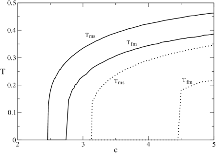
Figure 4: Critical temperatures as a function of the average connectivity $c$ for the ferromagnetic-paramagnetic phase transition ($T_{fm}$) and the spinodal line ($T_{ms}$). Parameters are: $p=3$, $J_{0}=0$ (solid); $p=4$, $J_{0}=0$ (dotted); For all lines $J=1$.

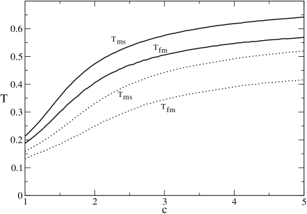
Figure 5: Critical temperatures as a function of the average connectivity $c$ for the ferromagnetic-paramagnetic phase transition ($T_{fm}$) and the spinodal line ($T_{ms}$). Parameters are: $p=3$, $J_{0}=0.1$ (solid); $p=4$, $J_{0}=0.1$ (dotted); For all lines $J=1$.

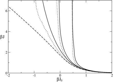
Figure 6: Phase transition lines in the $\beta J-\beta J_{0}$ plane for $p=3$ and different connectivities $c$: solid lines from right to left $c=1,3,10$. The dotted lines are the corresponding spinodal lines. The dashed line is for $c=\infty$.

Furthermore, we search for the transition lines in the $\beta J-\beta J_{0}$ plane. These transitions between $m\neq 0$ and $m=0$ are plotted in Fig. 6 for $p=3$, $\beta J>0$ and $c=1,3,10$ (solid lines), together with the spinodal lines (dotted lines) and the theoretical result for $c\rightarrow\infty$ (dashed line), which is solved analytically in Section IV. All transitions shown here are first-order. The ferromagnetic phase is situated to the right of the transition lines and increases substantially with growing $c$. For bigger values of $c$, the transitions approach the analytically derived $c=\infty$ result. Because $p$ is odd, the transition lines for $\beta J<0$ are found by reflection symmetry with respect to the $\beta J_{0}$ axis. Just as in the $p=2$ case, the small-world hypergraph has its ferromagnetic transition at finite temperatures for all non-zero values of $c$. Analogously to the $1+\infty$ dimensional case (see fig. 2), the ferromagnetic region decreases with increasing $p$, and disappears for $p\rightarrow\infty$.

Simulations have been performed for this small-world model with heat-bath dynamics and sequential updating. Our results in this perspective are somewhat limited by the nature of the phase transition: We are dealing with a very sparse system undergoing a first-order phase transition. Metastabilities will be present (as already indicated by the presence of the spinodal lines) and cause slow dynamics near the thermodynamic transition line. This in turn causes the system to show strong hysteresis effects. With these simulations we can look for the spinodal line by initializing the system in a fully magnetized state, and looking for the temperature where order disappears at long times. As a typical example the results for $p=3,c=3$ are plotted in Fig. 7 for $10^{4}$ spins and different numbers of iterations. Very good agreement with the spinodal line obtained with the population dynamics solution is found in the positive $\beta J_{0}$ region. When $J_{0}$ is negative however we do not find satisfactory results. This can be explained by the opposing forces at work in the system (ferromagnetic graph and antiferromagnetic chain), which will only slow the dynamics further down. We were unable to pinpoint the thermodynamic phase transitions with simulations due to the effects mentioned above. The simulations show some further evidence for glassy dynamics (very large spin-spin autocorrelation times) for lower temperatures, but a detailed discussion of such non-trivial glassy behavior is beyond the scope of the present work.

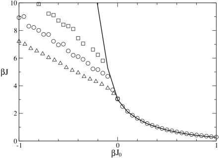
Figure 7: Phase transition lines in the $\beta J-\beta J_{0}$ plane for $p=3,c=3$. The solid line represents the spinodal line found by the population dynamics result. The triangles, circles and squares indicate the results of simulations with $10^{4}$ spins and, respectively, $2000,5\times 10^{4},5\times 10^{6}$ iterations per spin.

VI Discussion

In this paper, we have studied the thermodynamics of small-world hypergraphs consisting of sparse Poisson random graphs with $p$-spin interactions superimposed onto a one-dimensional Ising chain with nearest-neighbor interactions. Using a replica-symmetric transfer-matrix analysis and the population dynamics algorithm we have obtained the phase behavior of this system as a function of the short-range and long-range couplings. We find for $p\geq 3$ that all paramagnetic-ferromagnetic phase transitions are purely first order, in contrast with $p=2$ where also a second order phase transition occurs. For fixed $p$ and increasing connectivity $c$ the ferromagnetic phase increases substantially and the transition line converges to the analytically derived result for the $1+\infty$ dimensional model. For the latter the ferromagnetic region decreases for growing $p$. Using a bifurcation analysis we see that again, $p=2$ has also a second-order transition and the first-order transition occurs only for $\beta J_{0}\leq-0.275$.

Appendix: self-consistent equation for $\phi(x)$

In order to derive the self-consistent equation for $\phi(x)$ we insert (26) into the l.h.s. of (21) using (LABEL:T)

$$\sum_{\mbox{\boldmath$\tau$}}T_{\mbox{\boldmath$\sigma$},\mbox{\boldmath$\tau$}}[F]u_{0}(\mbox{\boldmath$\tau$})$$ (58)

$$= \sum_{\mbox{\boldmath$\tau$}}\exp\left(\beta J_{0}\sum_{\alpha}\sigma^{\alpha}\tau^{\alpha}+c\sum_{\mbox{\boldmath$\tau$}_{1}\ldots\mbox{\boldmath$\tau$}_{p-1}}\prod_{k=1}^{p-1}F(\mbox{\boldmath$\tau$}_{k})\left(e^{\frac{\beta J}{c}\sum_{\alpha}\tau_{1}^{\alpha}\ldots\tau_{p-1}^{\alpha}\sigma^{\alpha}}-1\right)\right)\int dx\>\phi(x)e^{\beta x\sum_{\alpha=1}^{n}\tau^{\alpha}}$$

$$= \sum_{\mbox{\boldmath$\tau$}}\int dx\>\phi(x)e^{\beta x\sum_{\alpha=1}^{n}\tau^{\alpha}}e^{\beta J_{0}\sum_{\alpha}\sigma^{\alpha}\tau^{\alpha}}e^{-c}\sum_{\mu=0}^{\infty}\left(\frac{c^{\mu}}{\mu!}\left(\sum_{\mbox{\boldmath$\tau$}_{1}\ldots\mbox{\boldmath$\tau$}_{p-1}}\prod_{k=1}^{p-1}F(\mbox{\boldmath$\tau$}_{k})e^{\frac{\beta J}{c}\sum_{\alpha}\tau_{1}^{\alpha}\ldots\tau_{p-1}^{\alpha}\sigma^{\alpha}}\right)^{\mu}\right)$$ (59)

$$= \left(\prod_{\alpha=1}^{n}\sum_{\gamma=\pm 1}\int dx\>\phi(x)e^{\beta x\gamma+\beta J_{0}\sigma^{\alpha}\gamma}\right)\sum_{\mu=0}^{\infty}\left(\frac{e^{-c}c^{\mu}}{\mu!}\sum_{\{\mbox{\boldmath$\tau$}_{k}^{\nu}\}_{k\leq p-1}^{\nu\leq\mu}}\prod_{\nu=1}^{\mu}\left[\prod_{k=1}^{p-1}F(\mbox{\boldmath$\tau$}_{k}^{\nu})\right]e^{\frac{\beta J}{c}\sum_{\alpha}\tau_{1}^{\nu,\alpha}\ldots\tau_{p-1}^{\nu,\alpha}\sigma^{\alpha}}\right)$$ (60)

In the transition to (59) we have used that $F(\mbox{\boldmath$\psi$})$ is normalised to separate the term $e^{-c}$. We then have expanded the outermost of the remaining double exponential into a series. In (60) we have written the powers as a product over a new replica index $\nu$. The vectors $\tau$ now have two replica indices. We also note that a poissonian factor appears. At this point we insert Eq. (25) to obtain

$$\sum_{\mbox{\boldmath$\tau$}}T_{\mbox{\boldmath$\sigma$},\mbox{\boldmath$\tau$}}[F]u_{0}(\mbox{\boldmath$\tau$}) = \left(\prod_{\alpha=1}^{n}\sum_{\gamma=\pm 1}\int dx\>\phi(x)e^{\beta x\gamma+\beta J_{0}\sigma^{\alpha}\gamma}\right)$$ (61)

$$\times\sum_{\mu=0}^{\infty}\left(\frac{e^{-c}c^{\mu}}{\mu!}\sum_{\{\mbox{\boldmath$\tau$}_{k}^{\nu}\}_{k\leq p-1}^{\nu\leq\mu}}\prod_{\nu=1}^{\mu}\left[\prod_{k=1}^{p-1}\int dh_{k}^{\nu}\>W(h_{k}^{\nu})\prod_{\alpha=1}^{n}\frac{e^{\beta h_{k}^{\nu}\tau_{k}^{\nu,\alpha}}}{2\cosh(\beta h_{k}^{\nu})}\right]e^{\frac{\beta J}{c}\sum_{\alpha}\tau_{1}^{\nu,\alpha}\ldots\tau_{p-1}^{\nu,\alpha}\sigma^{\alpha}}\right)$$

$$= \sum_{\mu=0}^{\infty}\left(\frac{e^{-c}c^{\mu}}{\mu!}\left[\prod_{\nu=1}^{\mu}\prod_{k=1}^{p-1}\int dh_{k}^{\nu}\>\frac{W(h_{k}^{\nu})}{(2\cosh(\beta h_{k}^{\nu}))^{n}}\right]\int dx\>\phi(x)\right.$$

$$\times\left.\prod_{\alpha=1}^{n}\left(\sum_{\gamma=\pm 1}e^{\beta\gamma(x+J_{0}\sigma^{\alpha})}\right)\prod_{\nu=1}^{\mu}\sum_{\gamma_{1}\ldots\gamma_{p-1}}e^{\beta\sum_{k=1}^{p-1}h_{k}^{\nu}\gamma_{k}+\frac{\beta J}{c}\gamma_{1}\ldots\gamma_{p-1}\sigma^{\alpha}}\right)$$

We now focus on the second line of the last equation

$$\prod_{\alpha=1}^{n}\left(\sum_{\gamma=\pm 1}e^{\beta\gamma(x+J_{0}\sigma^{\alpha})}\right)\prod_{\nu=1}^{\mu}\sum_{\gamma_{1}\ldots\gamma_{p-1}}e^{\beta\sum_{k=1}^{p-1}h_{k}^{\nu}\gamma_{k}+\frac{\beta J}{c}\gamma_{1}\ldots\gamma_{p-1}\sigma^{\alpha}}$$ (62)

$$= \exp\left(\sum_{\alpha=1}^{n}\log\left(G^{R}_{\sigma^{\alpha}}(x,\{h_{k}^{\nu}\})\right)\right)$$

$$= \exp\left(\sum_{\alpha=1}^{n}\sum_{s=\pm 1}\frac{1}{2}(1+s\sigma_{\alpha})\log\left(G^{R}_{s}(x,\{h_{k}^{\nu}\})\right)\right)$$

$$= \exp\left(\frac{1}{2}\left(\sum_{s=\pm 1}s\log\left(G^{R}_{s}(x,\{h_{k}^{\nu}\})\right)\right)\sum_{\alpha=1}^{n}\sigma_{\alpha}+\frac{n}{2}\sum_{s=\pm 1}\log\left(G^{R}_{s}(x,\{h_{k}^{\nu}\})\right)\right)$$

with (recall equation (32))

$$G^{R}_{\sigma}(x,\{h_{k}^{\nu}\})=\left(\sum_{\gamma=\pm 1}e^{\beta\gamma(x+J_{0}\sigma)}\right)\prod_{\nu=1}^{\mu}\sum_{\gamma_{1}\ldots\gamma_{p-1}}e^{\beta\sum_{k=1}^{p-1}h_{k}^{\nu}\gamma_{k}+\frac{\beta J}{c}\gamma_{1}\ldots\gamma_{p-1}\sigma}$$ (63)

We take the limit $n\rightarrow 0$ in (62) and replace the last line of (61) with this limit

$$\sum_{\mbox{\boldmath$\tau$}}T_{\mbox{\boldmath$\sigma$},\mbox{\boldmath$\tau$}}[F]u_{0}(\mbox{\boldmath$\tau$}) = \sum_{\mu=0}^{\infty}\left(\frac{e^{-c}c^{\mu}}{\mu!}\left[\prod_{\nu=1}^{\mu}\prod_{k=1}^{p-1}\int dh_{k}^{\nu}\>\frac{W(h_{k}^{\nu})}{(2\cosh(\beta h_{k}^{\nu}))^{n}}\right]\int dx\>\phi(x)\right.$$ (64)

$$\times\left.\exp\left(\frac{1}{2}\left(\sum_{s=\pm 1}s\log\left(G^{R}_{s}(x,\{h_{k}^{\nu}\})\right)\right)\sum_{\alpha=1}^{n}\sigma_{\alpha}\right)\right)$$

$$= \int dx^{\prime}\sum_{\mu=0}^{\infty}\left(\frac{e^{-c}c^{\mu}}{\mu!}\left[\prod_{\nu=1}^{\mu}\prod_{k=1}^{p-1}\int dh_{k}^{\nu}\>\frac{W(h_{k}^{\nu})}{(2\cosh(\beta h_{k}^{\nu}))^{n}}\right]\int dx\>\phi(x)\right.$$

$$\times\left.\delta\left[x^{\prime}-\frac{1}{2\beta}\left(\sum_{s=\pm 1}s\log\left(G^{R}_{s}(x,\{h_{k}^{\nu}\})\right)\right)\right]\exp\left(\beta x^{\prime}\sum_{\alpha=1}^{n}\sigma_{\alpha}\right)\right)$$

This expression is now of the form (26) and identifying terms leads to

$$\lambda_{0}\phi(x^{\prime}) = \sum_{\mu=0}^{\infty}\left(\frac{e^{-c}c^{\mu}}{\mu!}\left[\prod_{\nu=1}^{\mu}\prod_{k=1}^{p-1}\int dh_{k}^{\nu}\>W(h_{k}^{\nu})\right]\int dx\>\phi(x)\delta\left[x^{\prime}-\frac{1}{2\beta}\left(\sum_{s=\pm 1}s\log\left(G^{R}_{s}(x,\{h_{k}^{\nu}\})\right)\right)\right]\right)$$

where we have used additionally that $(2\cosh(\beta h_{k}^{\nu}))^{n}\rightarrow 1$ when $n\rightarrow 0$.

This equation can be simplified further as follows

$$G^{R}_{s}(x,\{h_{k}^{\nu}\}) = \left(\sum_{\gamma=\pm 1}e^{\beta\gamma(x+J_{0}\sigma)}\right)\prod_{\nu=1}^{\mu}\sum_{\gamma_{1}\ldots\gamma_{p-1}}e^{\beta\sum_{k=1}^{p-1}h_{k}^{\nu}\gamma_{k}+\frac{\beta J}{c}\gamma_{1}\ldots\gamma_{p-1}\sigma}$$ (65)

$$= 4\cosh\left(\beta(x+J_{0}\sigma)\right)\prod_{\nu=1}^{\mu}\sum_{\gamma_{2}\ldots\gamma_{p-1}}\cosh\left(\beta h_{1}^{\nu}+\frac{\beta J}{c}\gamma_{2}\ldots\gamma_{p-1}\sigma\right)e^{\beta\sum_{k=2}^{p-1}h_{k}^{\nu}\gamma_{k}}$$

$$= 4\exp\left(\frac{1}{2}\log(\cosh(\beta h_{1}^{\nu}+\frac{\beta J}{c})\cosh(\beta h_{1}^{\nu}-\frac{\beta J}{c}))\right)\cosh\left(\beta(x+J_{0}\sigma)\right)$$

$$\times\prod_{\nu=1}^{\mu}\sum_{\gamma_{2}\ldots\gamma_{p-1}}\exp\left(\gamma_{2}\ldots\gamma_{p-1}\sigma\>{\rm{atanh}}(\tanh(\beta h_{1}^{\nu})\tanh(\frac{\beta J}{c}))\right)e^{\beta\sum_{k=2}^{p-1}h_{k}^{\nu}\gamma_{k}}$$

$$= C(h_{1}^{\nu},h_{2}^{\nu},\ldots,h_{p-1}^{\nu},J)\exp\left(\sum_{\nu=1}^{\mu}\sigma\>{\rm{atanh}}\left(\tanh(\frac{\beta J}{c})\prod_{k=1}^{p-1}\tanh(\beta h_{k}^{\nu})\right)\right)$$

with $C(h_{1}^{\nu},h_{2}^{\nu},\ldots,h_{p-1}^{\nu},J)$ a function depending only on $h_{1}^{\nu},h_{2}^{\nu},\ldots,h_{p-1}^{\nu},J$ and $\beta$. We finally arrive at

$$\frac{1}{2\beta}\left(\sum_{s=\pm 1}s\log\left(G^{R}_{s}(x,\{h_{k}^{\nu}\})\right)\right)$$ (66)

$$= \frac{1}{\beta}\left[\sum_{\nu=1}^{\mu}{\rm{atanh}}\left(\tanh(\frac{\beta J}{c})\prod_{k=1}^{p-1}\tanh(\beta h_{k}^{\nu})\right)+{\rm{atanh}}\left(\tanh(\beta x)\tanh(\beta J_{0})\right)\right]$$

In this way we have obtained the self-consistent equation (28) for $\phi(x)$. The equation for $\chi(x)$ can be derived in an analogous way.

From these equations we can also find the largest eigenvalue $\lambda_{0}$. Keeping the factor of order $n$ in (62) we end up with the following equation

$$\lambda_{0}\phi(x^{\prime}) = \sum_{\mu=0}^{\infty}\frac{e^{-c}c^{\mu}}{\mu!}\left[\prod_{\nu=1}^{\mu}\prod_{k=1}^{p-1}\int dh_{k}^{\nu}\>\frac{W(h_{k}^{\nu})}{(2\cosh(\beta h_{k}^{\nu}))^{n}}\right]\int dx\>\phi(x)$$ (67)

$$\times\delta\left[x^{\prime}-\frac{1}{2\beta}\left(\sum_{s=\pm 1}s\log\left(G^{R}_{s}(x,\{h_{k}^{\nu}\})\right)\right)\right]\exp\left(\sum_{s=\pm 1}\frac{n}{2}\left(\log\left(G^{R}_{s}(x,\{h_{k}^{\nu}\})\right)\right)\right)$$

When we integrate both sides over $x^{\prime}$ and expand the last exponential we find equation (31).

References

- (1) A. Pekalski, Phys. Rev. E 64, 057104 (2001).
- (2) M. Girvan and M.E.J. Newman, Proc. Natl. Acad. Sci. U.S.A. 99, 7821 (2002).
- (3) L. Siming et al, Science 303, 540 (2004).
- (4) A.-L. Barabási and Z.N. Oltvai, Nat. Rev. Gen. 5, 101 (2004).
- (5) M.E.J. Newman, Proc. Natl. Acad. Sci. U.S.A. 98, 404 (2002).
- (6) A. Barrat and M. Weigt, Eur. Phys. J. B 13, 547 (2000).
- (7) T. Nikoletopoulos, A. C. C. Coolen, I. Pérez Castillo, N. S. Skantzos, J. P. L. Hatchett and B. Wemmenhove, J. Phys. A: Math. Gen. 37, 6455 (2004).
- (8) R. Albert and A-L Barabási, Rev. Mod. Phys. 74, 47 (2002).
- (9) M.E.J. Newman, SIAM Rev. 45, 167 (2003).
- (10) Duncan J Watts, Small Worlds: The Dynamics of Networks between Order and Randomness (Princeton University Press, Princeton, 2003).
- (11) S.N. Dorogovtsev and J.F.F. Mendes, Evolution of Networks: From Biological Nets to the Internet and WWW (Oxford University Press, London, 2003).
- (12) A-L Barabási, Linked: The New Science of Networks (Oxford University Press, London, 2002).
- (13) E Ramadan, A Tarafdar, and A Pothen, 18th International Parallel and Distributed Processing Symposium (IPDPS’04) - Workshop 9 p. 189b
- (14) A. Wagner and D. A. Fell, Proc. R. Soc. Lond. B 268 1803-1810 (2001)
- (15) S. Franz, M. Mézard, F. Ricci-Tersenghi, M. Weigt, and R. Zecchina, Europhys. Lett. 55, 465 (2001).
- (16) A. Barrat and R. Zecchina, Phys. Rev. E 59, 1299 (1999).
- (17) F. Ricci-Tersenghi, M. Weigt and R. Zecchina, Phys. Rev. E 63, 026702 (2001).
- (18) R. Heylen, N.S. Skantzos, J. Busquets Blanco and D. Bollé, Phys. Rev. E 73, 016138 (2006).
- (19) M. Mézard and G. Parisi, Eur. Phys. J. B 20, 217 (2001).
- (20) N.S. Skantzos and A.C.C. Coolen, J. Phys. A: Math. Gen. 33, 5785 (2000).
- (21) M. Kardar, Phys. Rev. 28, 244 (1983).
- (22) M. Mézard, G. Parisi and M.A. Virasoro, Spin Glass Theory and Beyond (World Scientific, Singapore, 1987).