Quantum Monte Carlo study for multiorbital systems
with preserved spin and orbital rotational symmetries

Abstract

We propose to combine the Trotter decomposition and a series expansion of the partition function for Hund’s exchange coupling in a quantum Monte Carlo (QMC) algorithm for multiorbital systems that preserves spin and orbital rotational symmetries. This enables us to treat the Hund’s (spin-flip and pair-hopping) terms, which is difficult in the conventional QMC method. To demonstrate this, we first apply the algorithm to study ferromagnetism in the two-orbital Hubbard model within the dynamical mean-field theory (DMFT). The result reveals that the preservation of the SU(2) symmetry in Hund’s exchange is important, where the Curie temperature is grossly overestimated when the symmetry is degraded, as is often done, to Ising (Z₂). We then calculate the $t_{2g}$ spectral functions of Sr₂RuO₄ by a three-band DMFT calculation with tight-binding parameters taken from the local density approximation with proper rotational symmetry.

I Introduction

As was pointed out by Slater as early as in the 1930s,s36 the intra-atomic (Hund’s) exchange interaction is of great importance for ferromagnetism in transition metals. Also the intensive study of transition-metal oxides—fueled by the discovery of high-temperature superconductivity—revealed the pivotal role of orbitals and Hund’s exchange, not only for ferromagnetism but, e.g., also for the metal-insulator transition if98 ; an02 ; l03 ; kk04 ; ik05 ; mg05 ; pb05 ; kk05 ; ah05 and unconventional superconductivity.t00 ; h04 ; sa04

For studying such correlation effects in multiorbital systems, the dynamical mean-field theorymv89 ; gk96 (DMFT) is one of the most successful methods. It takes into account temporal fluctuations but neglects spatial ones, and is known to describe the Mott-Hubbard transition.gk96 Recently, the multiorbital Mott-Hubbard transition has been studied most intensively by DMFT, pb05 ; an02 ; l03 ; kk04 ; ik05 ; mg05 ; kk05 ; ah05 showing that the correct symmetry of the exchange coupling is essential, in particular, close to and at the Mott-Hubbard transition.

Also for realistic material calculations, multiorbital DMFT is important. In particular, the so-called local density approximation (LDA)+DMFT methodap97 allows for calculating strong correlations in materials from first principles, and it has become one of the most active fields in solid state physics.ks05 In this method, DMFT solves a model constructed from band structure obtained by the local density approximation. Since materials such as transition-metal oxides usually have several orbitals around $E_{F}$, the model is, in general, a multiorbital one. This multiorbital Hubbard model hence consists of the intra- and interorbital Coulomb interactions $U$ and $U^{\prime}$, Hund’s-exchange and the pair-hopping interactions $J$, as well as the one-electron hoppings obtained from the LDA.

DMFT maps the model self-consistently onto an effective impurity model which includes the same on-site interactions on an impurity site and an infinite number of bath sites, which are coupled to the impurity site through a hybridization (hopping). This impurity problem has to be solved numerically: For multiorbital models, the exact diagonalizationck94 (ED) and the Hirsch-Fye quantum Monte Carlo (HFQMC) method hf85 ; gk96 are the most widely employed nonperturbative impurity solvers. Both ED and HFQMC methods have their pros and cons and are hence favorable in different situations.

ED has the advantage that it can easily handle all the multiorbital interactions including Hund’s coupling and the pair-hopping term. However, it is severely restricted in the number of bath sites, even in the Lanczos implementations which can take into account most bath sites for $T=0$ or very low temperatures. cm05 Since it cannot treat so many sites (and orbitals), DMFT (ED) studies have been usually limited to two-orbital systems.

On the other hand, HFQMC simulation can handle not only two but more orbitals and, in contrast to ED, also produces continuous spectra. The former is important since there are various intriguing systems having three or more orbitals, especially $t_{2g}$ electron, perovskite-type transition-metal oxides, exemplified by the spin-triplet superconductor. ${\rm Sr_{2}RuO_{4}}$mm03 The continuous spectra are crucial for comparing with experiments, e.g., photoemission spectroscopy. For these reasons the HFQMC method has been by far the most widely employed impurity solver as far as LDA+DMFT is concerned.

In most DMFT HFQMC studies,remark1 however, only the Ising ($z$) component of Hund’s exchange coupling has been considered, with the pair-hopping term neglected. The reason is that the standard Hubbard-Stratonovich transformationh83 is only applicable to the density-density part ($\hat{H}_{U}$) of the interactions and something else is required for the $x$ and $y$ components of Hund’s coupling and the pair-hopping interaction ($\hat{H}_{J}$). A straightforward decoupling of $\hat{H}_{J}$ leads to a very severe sign problem,hv98 making such QMC calculations virtually impossible.

In order to take into account $\hat{H}_{J}$, we previously proposed a transformation with a real and discrete auxiliary field for these terms in two-orbital systems.sa04 ; h04 So far, $s$-wave superconductivitysa04 and the orbital-selective Mott transitionkk05 ; ah05 have been investigated with our transformation.

Despite these successes, some problems remain to be solved. First, it is still difficult to treat more than two orbitals: Since the exponential of $\hat{H}_{J}$ is not equal to the product of the exponentials of the distinct two-orbital parts $\hat{H}_{J}^{mm^{\prime}}$ ($m$ and $m^{\prime}$ denote orbitals),remark2 we cannot decouple $\hat{H}_{J}$ for three or more orbitals by the simple product of two-orbital parts. Second, the fermionic sign problemhv98 caused by $\hat{H}_{J}$ prevents us from studying low temperatures.

In the present paper we propose and show that these difficulties are greatly remedied by employing a perturbation series expansion (PSE), separating out the problematic $\hat{H}_{J}$ term. It should be noted that the method is numerically exact (and nonperturbative). Also, the method is easily implemented, since our updating algorithm for sampling weights and Green’s function is basically the same as the Hirsch-Fye algorithm, with the differences being only for a factor multipling the weights and an additional value for the auxiliary field. While we focus here on DMFT, i.e., QMC simulations for impurity problems, the same ideas can be employed also for the lattice QMC method.

The auxiliary-field QMC method based on PSE for electron systems was first proposed by Rombouts et al.rh99 These authors applied PSE to the finite-size single-orbital Hubbard model and succeeded in obtaining results without time-discretization errors with less computational time than the conventional, Trotter-decomposition algorithm.bs81 Although the method uses PSE, it counts all the contributions of the interaction since the perturbation order taken into account is higher than the maximum order of the samples above which the weight is virtually zero. So the scheme is essentially nonperturbative. Rubtsov et al. rl04 proposed another algorithm to evaluate the series expansion of the partition function and applied it to solve the DMFT equations. It does not involve any auxiliary fields but uses Wick’s theorem. Recently Werner et al. wc05 proposed to use a perturbation expansion starting from the strong-coupling limit.

In previous work,sa06 we extended Rombouts’ algorithm to the multiorbital Hubbard Hamiltonian, using a similar transformation as in Ref. sa04, [Eq. (3)] for $\hat{H}_{J}$, i.e., we expanded the Boltzmann factor (operator) with respect to the total interaction $\hat{H}_{U}+\hat{H}_{J}$ shifted by a constant. Then, we discretized the imaginary time $\beta=L\Delta\tau$ and used a Hirsch-Fye-like updating algorithm for solving the impurity model in the DMFT context. Although the method significantly relaxes the sign problem and allows, in principle, for more than two orbitals, it turned out that the calculations are too heavy at low temperatures or for strong couplings, especially for more than two orbitals. That is because the computational effort increases with the perturbation orders appearing in the Monte Carlo samples. This order can become very large (see Fig. 2) in multiorbital systems since there are many interactions: $(2M-1)M$ terms in $\hat{H}_{U}$ and $2(M-1)M$ terms in $\hat{H}_{J}$ per site, where $M$ is the number of orbitals.

To overcome this difficulty, we here propose to combine the HFQMC and the PSEQMC methods, i.e., to adopt the series expansion for $\hat{H}_{J}$, while the standard Trotter decomposition and Hubbard-Stratonovich decoupling are employed for $\hat{H}_{U}$. This algorithm enables us not only to handle three or more orbitals but also to reach much lower temperatures or stronger couplings than HFQMC (Ref. sa04, ) or PSEQMC calculations,sa06 even for the two-orbital Hubbard model.

In the following, we first introduce the multiorbital Hubbard model in Sec. II to turn to our algorithm in Sec. III, enclosing details for the weight factor in the Appendix. A validation and benchmarks are presented in Sec. IV. Applications to local spin moments and to ferromagnetism in the two-orbital Hubbard model along with an application to Sr₂RuO₄ are discussed in Sec. V. Section VI summarizes the paper and gives an outlook.

II Model

The $M$-orbital Hubbard Hamiltonian reads

$$\hat{H} \equiv\hat{H}_{0}+\hat{H}_{U}+\hat{H}_{J},$$ (1)

$$\hat{H}_{0} \equiv-t\sum_{ij\sigma}\sum_{m=1}^{M}c_{im\sigma}^{\dagger}c_{jm\sigma}-\mu\sum_{im\sigma}n_{im\sigma},$$

$$\hat{H}_{U} \equiv U\sum_{i,m}\left(n_{im\uparrow}n_{im\downarrow}-\frac{n_{im\uparrow}+n_{im\downarrow}}{2}\right)$$

$$+U^{\prime}\sum_{i,m<m^{\prime},\sigma}\left(n_{im\sigma}n_{im^{\prime}-\sigma}-\frac{n_{im\sigma}+n_{im^{\prime}-\sigma}}{2}\right)$$

$$+(U^{\prime}-J)\sum_{i,m<m^{\prime},\sigma}\left(n_{im\sigma}n_{im^{\prime}\sigma}-\frac{n_{im\sigma}+n_{im^{\prime}\sigma}}{2}\right),$$

$$\hat{H}_{J} \equiv\sum_{m<m^{\prime}}\hat{H}_{J}^{mm^{\prime}}$$

$$\equiv J\sum_{i,m<m^{\prime}}(c_{im\uparrow}^{\dagger}c_{im^{\prime}\downarrow}^{\dagger}c_{im\downarrow}c_{im^{\prime}\uparrow}$$

$$\hskip 45.0pt+c_{im\uparrow}^{\dagger}c_{im\downarrow}^{\dagger}c_{im^{\prime}\downarrow}c_{im^{\prime}\uparrow}+{\rm H.c.}),$$

where $c_{im\sigma}^{\dagger}(c_{im\sigma})$ creates (annihilates) an electron with spin $\sigma$ in orbital $m$ at site $i$, and $n_{im\sigma}\equiv c_{im\sigma}^{\dagger}c_{im\sigma}$. $\hat{H}_{0}$ describes the hopping of electrons between two neighboring sites $\langle ij\rangle$, which we assume, unless otherwise indicated, to be orbital independent. $\hat{H}_{U}$ is defined to be all the density-density interactions, i.e., the intraorbital ($U$) and interorbital ($U^{\prime}$) Coulomb interactions and the $z$ (or Ising) component of Hund’s coupling $J$. By contrast, $\hat{H}_{J}$ takes care of the terms that cannot be written as density-density interactions, which consist of the $x$ and $y$ component of Hund’s coupling as well as the pair-hopping interaction (second term), in which two electrons in an orbital transfer to other orbitals. The Hamiltonian is rotationally invariant not only in spin space but also in real (orbital) space if we satisfy the condition $U\!=\!U^{\prime}\!+\!2J$, which comes from the symmetry preserved between the Coulombic matrix elements for orbitals in a central field. We postulate the rotational invariance henceforth.

In the DMFT approximation, the Hamiltonian (1) is approximated by an impurity problem where the interactions $\hat{H}_{U}$ and $\hat{H}_{J}$ are restricted to a test atom (the impurity) embedded in the systems; and $\hat{H}_{0}$ describes the coupling to a noninteracting bath which has to be determined self-consistently.remark3 When we develop our algorithm in the next section, $\hat{H}_{0}$, $\hat{H}_{J}$, and $\hat{H}_{U}$ denote these terms of the impurity model, but the same ideas can also be applied for lattice QMC simulations of the Hubbard model.

III (Trotter + Series-expansion) Method

We start with the series expansion of the Boltzmann factor for continuous time after Ref. rh99, . However, here we perform this only for $\hat{H}_{J}$, i.e.,

$$e^{\gamma-\beta\hat{H}}=e^{-\beta(\hat{H}_{0}+\hat{H}_{U})+\gamma-\beta\hat{H}_{J}}$$

$$= e^{-\beta(\hat{H}_{0}+\hat{H}_{U})}+\sum_{k=1}^{\infty}\int_{0}^{1}dt_{k}\cdots\int_{0}^{t_{2}}dt_{1}\prod_{i=1}^{k}$$

$$\left[e^{-t_{i}\beta(\hat{H}_{0}+\hat{H}_{U})}(\gamma-\beta\hat{H}_{J})e^{t_{i}\beta(\hat{H}_{0}+\hat{H}_{U})}\right]e^{-\beta(\hat{H}_{0}+\hat{H}_{U})},$$

where we have shifted the Boltzmann factor by a constant $\gamma$ for $\beta\hat{H}_{J}$ to apply the auxiliary-field transformation Eq. (9) below.

Now we discretize the imaginary-time integrals and with the notation $\hat{X}_{1}\equiv\gamma-\beta\hat{H}_{J}$, Eq. (III) equals

$$e^{-\beta(\hat{H}_{0}+\hat{H}_{U})}+\sum_{k=1}^{\infty}L^{-k}\sum_{j_{k}=1}^{L}\cdots\sum_{j_{1}=1}^{j_{2}}\prod_{i=1}^{k}$$

$$\left[e^{-\frac{j_{i}}{L}\beta(\hat{H}_{0}+\hat{H}_{U})}\hat{X}_{1}e^{\frac{j_{i}}{L}\beta(\hat{H}_{0}+\hat{H}_{U})}\right]e^{-\beta(\hat{H}_{0}+\hat{H}_{U})}+O(\Delta\tau).$$

We now show that this sum can be rewritten as

$$\sum_{s_{1},\cdots,s_{L}}^{0,1}F(k;s_{1},s_{2},\cdots,s_{L})\prod_{i=1}^{L}[e^{-\Delta\tau(\hat{H}_{0}+\hat{H}_{U})}\hat{X}_{s_{i}}]$$

$$+O(\Delta\tau),$$ (4)

where $F$ is a positive weight factor, $k\equiv\sum_{i=1}^{L}s_{i}$, and $\hat{X}_{0}\equiv 1$. To obtain the representation  (III), we first cut off the $k$ summation in Eq. (III) at $L$. This cutoff is justified if $L$ is taken to be greater than the maximum perturbation order $k_{max}$ (defined and displayed below) appearing in the Monte Carlo samples, so that there are no contributions from higher-order terms. In practice, we can make $L$ much larger than $k_{max}$ (see Fig.2 below): $k_{max}$ depends on Hund’s coupling $J$, where $J$ is physically not so large, whereas we can choose $L$ to satisfy $L>\beta U$.

Second, we replace those terms having consecutive $\hat{X}_{1}$’s in Eq. (III) by proximate terms including only one $\hat{X}_{1}$’s per imaginary time interval $\Delta\tau$. For example, $\cdots\hat{X}_{1}\hat{X}_{1}e^{-\Delta\tau(\hat{H}_{0}+\hat{H}_{U})}\cdots$ is replaced by $\cdots\hat{X}_{1}e^{-\Delta\tau(\hat{H}_{0}+\hat{H}_{U})}\hat{X}_{1}\cdots$. This replacement reduces the number of possible configurations remarkably and casts the summation (III) into the form (III) similar to the Trotter decomposition, which enables us to employ their standard Hirsch-Fye algorithm with only a slightly more complicated auxiliary field at each time slice. The error of this approximation (commutation) is $O(\Delta\tau)$, i.e., of the same order as the time discretization, as long as the average order of the series expansion $\langle k\rangle$ is sufficiently smaller than $L$. This is simply because the terms having two or more consecutive $\hat{X}_{1}$’s rarely appear for $\langle k\rangle\ll L$. For example, consider the second order terms in Eq. (III). Altogether, there are $L(L+1)/2$ second-order terms, but only $L$ of these terms have two consecutive $\hat{X}_{1}$’s with the same imaginary time interval. Hence, the error is at most $O(2\Delta\tau/L)$. Similar argument for higher orders justify the replacement as long as $\langle k\rangle\ll L$. Since we do not simply drop the terms with two or more consecutive $\hat{X}_{1}$’s, but replace them by terms where the $\hat{X}_{1}$’s are shifted to neighboring imaginary time intervals, we have to multiply the Boltzmann factor by a factor $F$ to account for these replacements. The detailed derivation of $F$ is given in the Appendix.

Now, we separate out $\hat{H}_{U}$ in Eq. (III) using the Trotter decomposition as

$$e^{-\Delta\tau(\hat{H}_{0}+\hat{H}_{U})}=e^{-\Delta\tau\hat{H}_{0}}e^{-\Delta\tau\hat{H}_{U}}+O(\Delta\tau^{2}),$$ (5)

so that Eq. (III) has a similar form to the standard HFQMC method. The $e^{-\Delta\tau\hat{H}_{U}}$ term is then decoupled, as usual, into a sum of one-body exponentials with the Hubbard-Stratonovich transformation,

$$e^{-\Delta\tau V[n_{\alpha}n_{\beta}-\frac{n_{\alpha}+n_{\beta}}{2}]}=\frac{1}{2}\sum_{s}^{\pm 1}\left\{\begin{array}[]{l}e^{\lambda_{V}s(n_{\alpha}-n_{\beta})}\quad(V\geq 0),\\ e^{\lambda_{V}s(n_{\alpha}+n_{\beta}-1)+\frac{a}{2}}(V<0),\end{array}\right.$$ (8)

where $V$ stands for $U,U^{\prime},$ or $U^{\prime}-J$, $\lambda_{V}\equiv\ln(e^{|\Delta\tau V|/2}+\sqrt{e^{\left|\Delta\tau V\right|}-1})$. We have also displayed the case of attractive interaction, which we shall require when we do the procedure described in Ref. remark4, . Including all the $(2M-1)M$ interactions of density-density type, the decoupling for $e^{-\Delta\tau\hat{H}_{U}}$ is given by

$$e^{-\Delta\tau\hat{H}_{U}}=\sum_{P=1}^{N_{U}}\hat{Q}_{P}^{U},$$ (9)

$$\hat{Q}_{P}^{U}\equiv\frac{1}{N_{U}}\prod_{m=1}^{M}e^{\lambda_{U}p_{m}(n_{m\uparrow}-n_{m\downarrow})}$$

$$\times\prod_{m<m^{\prime},\sigma}e^{\lambda_{U^{\prime}}q_{\sigma}^{mm^{\prime}}(n_{m\sigma}-n_{m^{\prime},-\sigma})+\lambda_{U^{\prime}-J}r_{\sigma}^{mm^{\prime}}(n_{m\sigma}-n_{m^{\prime}\sigma})},$$

where $P(=1,...,N_{U}\equiv 2^{(2M-1)M})$ designates configurations of the auxiliary-field set $(\{p_{m}\},\{q_{\sigma}^{mm^{\prime}}\},\{r_{\sigma}^{mm^{\prime}}\})$ with $p_{m},q_{\sigma}^{mm^{\prime}},r_{\sigma}^{mm^{\prime}}=\pm 1$ denoting the fields for the $U$, $U^{\prime}$, and $U^{\prime}-J$ terms, respectively.

For $\hat{X}_{1}=\gamma-\beta\hat{H}_{J}$ in Eq. (III) we construct an auxiliary-field transformation as follows.sa06 ; rh98 We first decompose $\hat{X}_{1}$ into the sum of all distinct two-orbital parts as

$$\gamma-\beta\hat{H}_{J}=\!\sum_{m<m^{\prime}}[\gamma^{mm^{\prime}}-\beta\hat{H}_{J}^{mm^{\prime}}],\quad\gamma\equiv\!\sum_{m<m^{\prime}}\gamma^{mm^{\prime}}.$$ (10)

We then apply the decoupling

$$\gamma^{mm^{\prime}}-\beta\hat{H}_{J}^{mm^{\prime}}=$$

$$\frac{\gamma^{mm^{\prime}}-\beta J}{8}\!\!\sum_{s,t_{\uparrow},t_{\downarrow}}^{\pm 1}\prod_{\sigma}e^{\tilde{\lambda}_{J}[\sigma sf_{\sigma}^{mm^{\prime}}+t_{\sigma}(n_{m\sigma}+n_{m^{\prime}\sigma}-1)]}$$

to every pair of orbitals, where

$$f_{\sigma}^{mm^{\prime}} \equiv c_{m\sigma}^{\dagger}c_{m^{\prime}\sigma}+c_{m^{\prime}\sigma}^{\dagger}c_{m\sigma},$$

$$\tilde{\lambda}_{J} \equiv \frac{1}{2}\ln\frac{1+\kappa}{1-\kappa},$$

$$\kappa \equiv \sqrt{\frac{\beta J}{\gamma^{mm^{\prime}}}}<1.$$

Note that the difficulty in the HFQMC calculations coming from the noncommutativity of $\hat{H}_{J}^{mm^{\prime}}$’s is lifted in Eq. (10), so that we can readily deal with more than two orbitals. Combining Eqs. (10) and (III), we end up with

$$\gamma-\beta\hat{H}_{J}=\sum_{S=1}^{N_{J}}\hat{Q}_{S}^{J},$$ (12)

$$\hat{Q}_{S}^{J}\equiv\frac{\gamma^{mm^{\prime}}-\beta J}{8}\prod_{\sigma}e^{\tilde{\lambda}_{J}[\sigma sf_{\sigma}^{mm^{\prime}}+t_{\sigma}(n_{m\sigma}+n_{m^{\prime}\sigma}-1)]},$$

where $S[=1,...,N_{J}\equiv 4M(M-1)]$ corresponds to the set $(s,t_{\uparrow},t_{\downarrow})$ for all the $M(M-1)/2$ pairs of orbitals $(m,m^{\prime})$.

Collecting the addends from the decoupled $\hat{H}_{U}$ and $\hat{H}_{J}$ terms, we finally obtain

$$e^{\gamma-\beta\hat{H}}=\sum_{S_{1},\cdots,S_{L}}^{0,\cdots,N_{J}}F(k;\tilde{s}_{1},\tilde{s}_{2},...,\tilde{s}_{L})$$

$$\times\sum_{P_{1},\cdots,P_{L}}^{1,\cdots,N_{U}}\prod_{i=1}^{L}e^{-\Delta\tau\hat{H}_{0}}\hat{Q}_{P_{i}}^{U}\hat{Q}_{S_{i}}^{J}+O(\Delta\tau),$$ (13)

with $\hat{Q}_{0}^{J}\equiv 1$ and $\tilde{s_{i}}\equiv 0$ (for $S_{i}=0$) or 1 (otherwise).remark4 Note that because $F(0;0,...,0)=1$, the zeroth-order term in Eq. (III) reproduces the Hirsch-Fye algorithm with Ising-type Hund’s coupling.

Owing to the form of Eq. (III), we can apply the same algorithm as in HFQMC for Monte Carlo sampling. Even the updating equations for single spin flips are the same.

IV Benchmarks

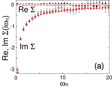
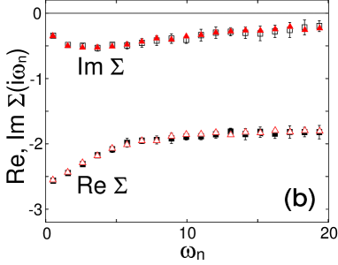
Figure 1: (Color online) Real and imaginary parts of the self-energy against the Matsubara frequency $\omega_{n}$ for the two-orbital Hubbard model for (a) an insulating case with $n=2,\beta=10,U^{\prime}=2,J=0.4$, and (b) a metallic case with $n=1,\beta=6,U^{\prime}=2,J=1$. Result with the Hirsch-Fye algorithm (Ref. sa04, ) is shown in black squares, and the present QMC result in red triangles.

As a benchmark, we compare in Fig. 1 the electron self-energy obtained from our algorithm with that from the HFQMC method of Ref. sa04, for the two-orbital Hubbard model. In these QMC methods the self-energy is obtained from Dyson’s equation, where Green’s function is calculated by averaging over QMC samples. We chose the hypercubic lattice with bandwidth $W=2$, and took $6\times 10^{6}$ Monte Carlo samples for both methods. We can see that the two results agree with each other within error bars for both (a) an insulating case at half filling $n=2$ with $\beta=10,U^{\prime}=2,J=0.4,L=100$, and (b) a metallic case at $n=1,\beta=6,U^{\prime}=2,J=1,L=64$. We notice, however, that the statistical error is much smaller in the present QMC approach than in the HFQMC one. This is because the number of negative signs is greatly reduced in the present scheme: The sign problem is mitigated. Quantitatively, the average sign in the QMC weights is 0.01 (0.03) for HFQMC methods while they are increased to 0.30 (0.50) in the present algorithm in case (a) [(b)]. This also implies that the present method can reach much lower temperatures. We note that, while $\gamma$ is arbitrary, we adopted in these and following calculations $\gamma-\beta V\sim 0.1-0.3$, which has turned out to reduce the computational time to some extent.

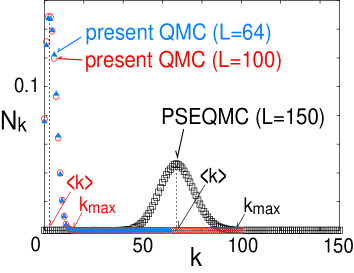
Figure 2: (Color online) The distribution $N_{k}$ of the order of perturbation $k$ for the two-orbital Hubbard model with $n=1.9,\beta=8,U^{\prime}=4,J=0.2$ obtained with the present algorithm ($L=64$ or $100$) and with the PSEQMC algorithm ($L=150$) (Ref. sa06, ).

Figure  2 depicts a typical distribution $N_{k}$ of the order of perturbation $k$ contributing in the Monte Carlo simulation for $n=1.9,\beta=8,U^{\prime}=4,J=0.2$. We can immediately see that the present algorithm has a peak in the distribution residing at much lower $k$ than for the PSEQMC approach.sa06 This is natural, since the present method uses the expansion only with respect to $\hat{H}_{J}$, while the PSEQMC method expands with respect to the total interaction $\hat{H}_{U}+\hat{H}_{J}$. We notice that the weight is virtually zero above a certain order, $k_{max}$, in actual calculations, so that, although the method is called perturbation expansion, it takes account of all orders in fact. We find that the maximum order in the distribution is $k_{max}\sim 100$ for the PSEQMC method, while $k_{max}\sim 15$ is much lowered for the present QMC method. This means that $L$ must be taken to be $>100$ for the PSEQMC method to take care of all orders, while $L>\beta U\sim 35$ suffices for the present algorithm to take care of all orders. Such a smaller value of $L$ dramatically reduces the computational effort in QMC simulations, which increases proportionately to $L^{3}$. Moreover, the average order $\langle k\rangle$ is about 4 for the present QMC, which means that the approximation employed to obtain the form (III) has only a very minor effect on the results, and hence is justifiable. This can also be confirmed from the fact that the results do not significantly depend on $L$.

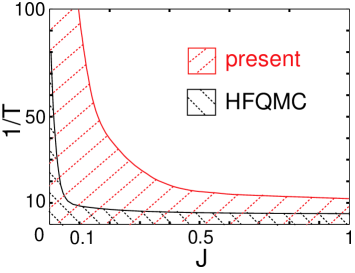
Figure 3: (Color online) Computable regions (hatched) in the $T$-$J$ parameter space that can be computed with the present and with the Hirsch-Fye QMC method (Ref. sa04, ) for the two-orbital Hubbard model with $U^{\prime}=4,W=2$. Here we define the computability by requiring average signs to be greater than 0.01.

Figure 3 shows the computable regions for the present QMC and for the HFQMC methods (Ref. sa04, ) when $\hat{H}_{J}$ is included. Here we define the region as computable when the average sign is greater than 0.01. We can see that a much wider parameter region becomes computable in the present algorithm than in the HFQMC method. For small $J\ (\lesssim 0.2)$, we can explore five to ten times lower temperatures. We attribute this improvement to the fact that $\hat{H}_{J}$ (which is the source of negative weights) appears $L$ times for every sample in the HFQMC method, while we have only $\langle k\rangle$ such terms on average in the present QMC algorithm.

V Applications

V.1 Local spin moment

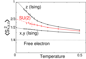
Figure 4: (Color online) Local spin moment for the two-orbital Hubbard model with SU(2)-type Hund’s and pair-hopping interactions as compared with Ising-type Hund’s coupling for $U^{\prime}=3,J=0.2,n=2$ (half filling) and the Gaussian density of states of width $W=2$. Solid lines are guides to the eye, dashed lines extrapolations, and the dotted line the local moment for free electrons.

Let us now turn to the first application of our algorithm. We first examine how results for the Hamiltonian with and without $\hat{H}_{J}$, i.e., with Z₂ and SU(2) symmetry, respectively, can differ. In Fig. 4, we show the temperature dependence of the local spin moment in the paramagnetic phase at half filling in the two-orbital Hubbard model for $U^{\prime}=3,J=0.2$ on a hypercubic lattice with bandwidth $W=2$. At these parameters, the system becomes insulating at zero temperature for both the Z₂ (Ising) and the SU(2) cases. The spin moments are defined by

$$\langle S_{z}^{2}\rangle =\frac{1}{4}\langle(\sum_{ms}\sigma n_{m\sigma})^{2}\rangle,$$ (14)

$$\langle S_{x}^{2}\rangle =\frac{1}{4}\langle(\sum_{m}c_{m\uparrow}^{\dagger}c_{m\downarrow}+c_{m\downarrow}^{\dagger}c_{m\uparrow})^{2}\rangle,$$ (15)

$$\langle S_{y}^{2}\rangle =-\frac{1}{4}\langle(\sum_{m}c_{m\uparrow}^{\dagger}c_{m\downarrow}-c_{m\downarrow}^{\dagger}c_{m\uparrow})^{2}\rangle=\langle S_{x}^{2}\rangle.$$ (16)

For the Ising case $\langle S_{z}^{2}\rangle$ is always larger than $\langle S_{x,y}^{2}\rangle$, while for the SU(2) case these components have the same value (within statistical error bars) as they should, which lies between the $\langle S_{z}\rangle$ and $\langle S_{x}\rangle,\langle S_{y}\rangle$ in the Ising case. As the temperature is lowered in the Ising case, $\langle S_{z}^{2}\rangle$ and $\langle S_{x,y}^{2}\rangle$ approach 1 and $\frac{1}{2}$, respectively, while for SU(2) symmetry both expectation values converge to $\frac{2}{3}$. This is easily understood by considering the fact that the ground state in the atomic limit is a doublet with $S_{z}=\pm 1$ in the Z₂ case, whereas it is a triplet with $S_{z}=0,\pm 1$ in the SU(2) case.

V.2 Ferromagnetism

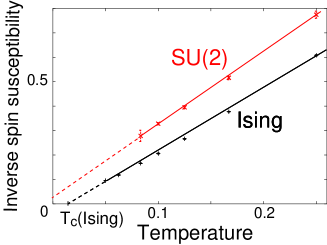
Figure 5: (Color online) Inverse spin susceptibility for the two-orbital Hubbard model with SU(2)-type Hund’s and pair-hopping interactions as compared with the Ising-type Hund’s coupling for $U^{\prime}=2.5,J=1$ with the semielliptical density of states of width $W=2$. The solid lines are guides to the eye, and the dashed lines extrapolations.

We now turn to the long-range ferromagnetic ordering, which reveals a more important difference between Z₂ and SU(2) symmetries as Fig. 5 shows. To this end, we have calculated the temperature dependence of the magnetic susceptibility in the two-orbital Hubbard model for $U^{\prime}=2.5,J=1,n=1.25$ with a semielliptical density of states of width $W=2$. The lattice susceptibilities are obtained here through the Bethe-Salpeter equation.gk96 The Curie temperature for the Hamiltonian with Ising-type Hund’s coupling is estimated by a Curie-Weiss extrapolation to be 0.01-0.02, in accordance with the previous results.hv98 In contrast, the present result shows that the inverse susceptibility does not intersect the horizontal axis, implying an absence of ferromagnetic transitions, for these parameters if the SU(2) symmetry of Hund’s exchange and the pair-hopping term are respected.

The result suggests that an Ising-type treatment of Hund’s coupling grossly overestimates the tendencies toward ferromagnetic ordering. Indeed, Ising-type DMFT calculations for manganites hv00 and iron lk01 gave Curie temperatures much higher than the experimental results. The present comparison indicates that the main reason for overestimating the Curie temperature in such calculations is not only the mean-field nature of DMFT but the incorrect symmetry of the Hund’s exchange. For an Ising-type Hund’s exchange, (local) transverse spin fluctuations, which are the main source of softening magnetic moments, are suppressed.

V.3 Quasiparticle density of states for ${\rm Sr_{2}RuO_{4}}$

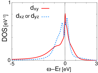
Figure 6: (Color online) Quasiparticle density of states for $t_{2g}$ orbitals in ${\rm Sr_{2}RuO_{4}}$, obtained by a simplified LDA+DMFT (QMC) calculation with three-orbital rotationally invariant Hamiltonian (1).

Finally we demonstrate that the present QMC method is actually applicable to realistic three-orbital systems. As an illustration, we take ${\rm Sr_{2}RuO_{4}}$, which can be treated as a ($t_{2g}$) three-orbital system, consisting of a wide two-dimensional band ($d_{xy}$) and two degenerate narrow one-dimensional bands ($d_{xz},d_{yz}$). The material belongs to an important family of transition-metal oxides where superconductivity,mm03 magnetism,cm66 and orbital-selective Mott transitionan02 ; l03 ; kk04 ; ik05 ; mg05 are discussed. To our knowledge, this is the first QMC calculation for a three-orbital system with SU(2)-symmetric Hund’s exchange and pair-hopping interaction.

Liebsch and Lichtenstein ll00 already obtained the quasiparticle density of states for this material with a simplified LDA+DMFT (HFQMC) calculation using the three-orbital Hamiltonian without $\hat{H}_{J}$ (i.e., an Ising-type treatment of Hund’s coupling). As a LDA input they constructed a tight-binding model that reproduces the LDA density of states. We have employed the same initial tight-binding model (for the density of states), the same number of $t_{2g}$ electrons per site ($n=3.7$), and the same interaction parameters $U^{\prime}=0.8\,$eV, $J=0.2\,$eV, but a somewhat higher temperature $T=25\,$meV.

The LDA+DMFT spectral functions, obtained with the maximum entropy method, are shown in Fig. 6. The quasi-two-dimensional (2D) $d_{xy}$ band has a van Hove singularity just above the Fermi energy $E_{F}$, while the quasi-1D $d_{xz}$ and $d_{yz}$ bands have broad peaks on both sides of $E_{F}$ and a small peak near $E_{F}$. Although these structures are similar to those of Liebsch and Lichtenstein, ll00 it may be due to the small value of $J$ employed here. In general, $\hat{H}_{J}$ can have a significant influence on quasiparticle spectra. We have obtained results substantially changed by $\hat{H}_{J}$, for example, enhancement of Kondo resonance by $\hat{H}_{J}$, for artificially elevated $U$, $U^{\prime}$, and $J$ (not shown here). Actually, values of $U$, $U^{\prime}$, and $J$ larger than those used here, as usually assumed for transition-metal oxides, were recently suggested for Sr₂RuO₄,pn06 and it will enhance the effect of $\hat{H}_{J}$.

VI Summary and Outlook

In summary, we have formulated a numerically exact auxiliary-field QMC scheme for the spin- and orbital-rotationally-invariant Hamiltonian (1) by combining series expansion and Trotter decomposition. We have implemented this algorithm for impurity models and employed it to solve the DMFT equations. The approach enables us not only to address three- (or more-)orbital systems but also to reach much lower temperatures than the previous QMC methods, which is the case with two-orbital systems as well.

The calculation of the magnetic susceptibility shows that an Ising treatment of Hund’s coupling overestimates tendencies towards ferromagnetism, which we attribute to neglected transversal spin fluctuations. In this sense the SU(2) symmetry in Hund’s exchange is indicated to be mandatory for an accurate study of magnetic phenomena with (LDA+)DMFT. We finally applied the present method to a realistic three-orbital system ${\rm Sr_{2}RuO_{4}}$, to demonstrate that the QMC algorithm can be employed for LDA+DMFT calculations.

Since we can apply the usual Hirsch-Fye updating algorithm with only minor changes in the additional values of the auxiliary field and a factor for the weights, the present scheme can be conveniently applied to multiorbital DMFT studies, especially for LDA+DMFT calculations requiring three orbitals. Although the fermionic sign problem still remains at low temperatures, we can reach much lower temperatures than before.sa04 Also, a combination of the present method with the projective QMC methodfh04 ; ah05 is very promising, which may provide an avenue for examining ground states, which is now under way.

Appendix

We derive here the factor $F(k;s_{1},s_{2},...,s_{L})$ $(s_{i}=0,1;k=\sum_{i=1}^{L}s_{i})$ for Eq. (III). We introduce this factor to account for the contribution from the terms with consecutive $\hat{X}_{1}$’s at the same imaginary-time interval in the sum (III). These terms have been replaced with terms having $\hat{X}_{1}$’s on proximate imaginary-time intervals in Eq. (III). In the following we abbreviate $e^{-\Delta\tau(\hat{H}_{0}+\hat{H}_{U})}$ as $h$, and $\hat{X}_{1}$ as $x$.

Central to our considerations are those terms that include a substring $xhxhx\cdots hx$ where $x$ and $h$ appear alternately $m$ and $m-1$ times, respectively, with $2\leq m\leq L$. This is because any term with consecutive $x$’s will be replaced with a term having such substrings. For example, $xxhhx\cdots hx$ and $xhxxh\cdots hx$ are both approximately the same as $xhxhx...hx$ [where commuting an $x$ and a $h$ yields an error $\sim O(\Delta\tau)$]. In general, we commute $x$’s and $h$’s until there are no consecutive $x$’s any longer. Hence, we end up with an alternation of $x$’s and $h$’s, i.e., an $xhxhx...hx$ substring. Because of these replacements, terms having such a substring have to be weighted more. In the following, we construct a rule for the replacement and weighting factor, avoiding a double counting.

Let us denote by $i$ a position (from the left) in a substring which consists of $m$ $x$’s and $(m-1)$ $h$’s altogether. We define $\alpha_{i}$ and $\beta_{i}$ as the number of $x$’s and $h$’s that are in $[1,i]$. All substrings having

$$\alpha_{i}\geq\beta_{i}\quad{\rm for\ all}\ i$$ (17)

will be replaced with $xhxhx...hx$ which has alternating $x$’s and $h$’s.

For example, for $m=2$ $xhx$ and $xxh$ will be replaced with $xhx$; for $m=3$, $xhxhx,xhxxh,xxhhx,xxhxh$ and $xxxhh$ will all be replaced with $xhxhx$. The condition (17) is necessary to avoid a double counting. However, the condition (17) excludes the substrings situated at the end of the imaginary time interval for which $\exists\ i^{\prime}$, so that $\alpha_{i^{\prime}}<\beta_{i^{\prime}}$. These terms are replaced with a substring $xhxhx\cdots hx$, where the last $x$ is at $L$, namely, only when the last $x$ is at $L$, does $xhxhx\cdots hx$ replace all the substrings having $m$ $x$’s and $(m-1)$ $h$’s, which requires a separate treatment ($c$ factors below).

A second factor to be taken into account is the correction of the volume in the imaginary-time integrals; namely, the weight for those terms having consecutive $x$’s at

$$j_{i}\neq j_{i+1}=j_{i+2}=\cdots=j_{i+l}\neq j_{i+l+1}$$ (18)

in the sum (III) should be reduced by a factor $\frac{1}{l!}$, since the imaginary times originally satisfy a relation

$$t_{i+1}<t_{i+2}<\cdots<t_{i+l}$$ (19)

in Eq. (III). Hence the volume for $l$ consecutive $x$ terms, as in Eq. (18), should be reduced to $\frac{L^{-l}}{l!}$.

Let us now introduce the quantity $b(i,j)$ for the weight (apart from the volume factor $L^{-j}$) of all the substrings having $i$ $h$’s and $j$ $x$’s. For $j$ consecutive $x$’s, we simply have the aforementioned $1/l!$ factor, i.e.,

$$b(0,j)=\frac{1}{j!}\quad{\rm for}\quad 0\leq j\leq L.$$ (20)

This is the starting point for the recurrence formula,

$$b(i,j)=\sum_{k=i}^{j}\frac{1}{(j-k)!}b(i\!-\!1,k)\ {\rm for}\ 1\leq i\leq j\leq L,$$ (21)

which arises from taking away the rightmost elements of the type $hxxx\cdots x$ with $(j-k)$ $x$’s from the substring of length $i+j$. At the end, the recurrance formula Eq. (21) yields the weighting factor $a_{i}$ for the substring ‘$xhxhx\cdots hx$’ with $m$ $x$’s and $m-1$ $h$’s:

$$a_{i}=b(i-1,i)=b(i,i)\quad{\rm for}\quad 1\leq i\leq L.$$ (22)

Only when the last $x$ in $xhxhx...hx$ is situated at the end of the imaginary-time interval ($L$) do we use the factor $c_{m}$ instead, which is obtained via the slightly different recurrence formula [see Fig. 7(b)],

$$d(0,j)=\frac{1}{j!}\quad{\rm for}\quad 0\leq j\leq L,$$

$$d(i,j)=\sum_{k=0}^{j}\frac{1}{(j-k)!}d(i\!-\!1,k)$$

$$\quad{\rm for}\quad 1\leq i\leq L-1\ {\rm and}\ 0\leq j\leq L,$$

$$c_{i}=d(i-1,i)\quad{\rm for}\quad 1\leq i\leq L.$$ (23)

From the $a$’s and $c$’s, the total weight $F$ is calculated by multiplying the contributions ${a_{m}}$ and ${c_{m}}$ from each $xhxhx...hx$-type substring in the Boltzmann factor and the volume $L^{-k}$. For example, for $L=8$,

$$F(2;1,1,0,0,0,0,0,0)=a_{2}L^{-2},$$

$$F(5;0,1,0,1,0,1,1,1)=c_{3}L^{-5},$$

$$F(6;1,0,1,1,0,1,1,1)=a_{2}c_{3}L^{-6}.$$ (24)

In the first example, the Boltzmann factor is $hxhxhhhhhh$. This array replaces itself and $hxxhhhhhhh$, which is weighted $\frac{1}{2!}$, and thereby the factor is $a_{2}=1+\frac{1}{2!}=\frac{3}{2}$ multiplied by $L^{-2}$. The second example corresponds to $hhxhhxhhxhxhx$, where the substring to be multiplied by a factor is only the last part $xhxhx$. Therefore the factor is $c_{3}L^{-5}$. In the last example $hxhhxhxhhxhxhx$, two substrings $xhx$ and $xhxhx$ are multiplied by $a_{2}$ and $c_{3}$, respectively. So the total factor is $a_{2}\times c_{3}L^{-6}$.

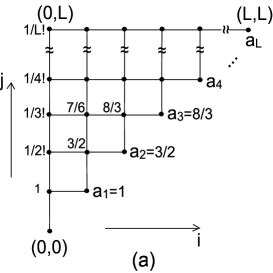
Figure 7: A schematic representation of the calculation of (a) $a_{m}$ and (b) $c_{m}$. The coordinates in the $i$ and $j$ directions represent the numbers of $h$ and $x$, respectively. The number at a point $(i,j)$ denotes (a) $b(i,j)$ and (b) $d(i,j)$, which are recursively calculated with Eq. (21) and (Appendix), respectively.

References

- (1) [] ∗ Present address: Condensed Matter Theory Laboratory, RIKEN, Wako, Saitama 351-0198, Japan.
- (2) J. C. Slater, Phys. Rev. 49, 537 (1936).
- (3) M. Imada, A. Fujimori, and Y. Tokura, Rev. Mod. Phys. 70, 1039 (1998); M. J. Rozenberg, Phys. Rev. B 55, R4855 (1997); J. E. Han, M. Jarrell, and D. L. Cox, ibid. 58, R4199 (1998); Y. no, R. Bulla, and M. Potthoff, ibid. 67, 035119 (2003).
- (4) Th. Pruschke and R. Bulla, Eur. Phys. J. B 44, 217 (2005).
- (5) V. I. Anisimov, I. A. Nekrasov, D. E. Kondakov, T. M. Rice, and M. Sigrist, Eur. Phys. J. B 25, 191 (2002)
- (6) A. Liebsch, Phys. Rev. Lett. 91, 226401 (2003); Phys. Rev. B 70, 165103 (2004)
- (7) A. Koga, N. Kawakami, T. M. Rice, and M. Sigrist, Phys. Rev. Lett. 92, 216402 (2004).
- (8) K. Inaba, A. Koga, S. Suga, and N. Kawakami, J. Phys. Soc. Jpn. 74, 2393 (2005); Phys. Rev. B 72, 085112 (2005); M. Ferrero, F. Becca, M. Fabrizio, and M. Capone, ibid. 72, 205126 (2005); C. Knecht, N. Blümer, and P. G. J. van Dongen, ibid. 72, 081103(R) (2005); A. Liebsch, Phys. Rev. Lett. 95, 116402 (2005); A. Koga, K. Inaba, and N. Kawakami, Prog. Theor. Phys. Suppl. 160, 253 (2005); S. Biermann, L. de’ Medici, and A. Georges, Phys. Rev. Lett. 95, 206401 (2005); P. G. J. van Dongen, C. Knecht, and N. Blümer, Phys. Status Solidi B 243, 116 (2006); A. Liebsch and T. A. Costi, Euro. Phys. J. B. 51, 523 (2006).
- (9) L. de’ Medici, A. Georges, and S. Biermann, Phys. Rev. B 72, 205124 (2005)
- (10) A. Koga, N. Kawakami, T. M. Rice, and M. Sigrist, Phys. Rev. B 72, 045128 (2005).
- (11) R. Arita and K. Held, Phys. Rev. B 72, 201102(R) (2005).
- (12) T. Takimoto, Phys. Rev. B 62, R14641 (2000); M. Capone, M. Fabrizio, C. Castellani, and E. Tosatti, Science 296, 2364 (2002); T. Hotta and K. Ueda, Phys. Rev. Lett. 92, 107007 (2004); Y. Yanase, M, Mochizuki, and M. Ogata, J. Phys. Soc. Jpn. 74, 430 (2005); M. Mochizuki, Y. Yanase, and M. Ogata, Phys. Rev. Lett. 94, 147005 (2005).
- (13) An alternative, continuous auxiliary field has been proposed by J. E. Han, Phys. Rev. B 70, 054513 (2004).
- (14) S. Sakai, R. Arita, and H. Aoki, Phys. Rev. B 70, 172504 (2004).
- (15) W. Metzner and D. Vollhardt, Phys. Rev. Lett. 62, 324 (1989).
- (16) A. Georges, G. Kotliar, W. Krauth, and M. J. Rozenberg, Rev. Mod. Phys. 68, 13 (1996).
- (17) V. I. Anisimov, A. I. Poteryaev, M. A. Korotin, A. O. Anokhin, and G. Kotliar, J. Phys.: Condens. Matter 9, 7359 (1997); A.I. Lichtenstein and M.I. Katsnelson, Phys. Rev. B 57, 6884 (1998).
- (18) G. Kotliar, S. Y. Savrasov, K. Haule, V. S. Oudovenko, O. Parcollet, and C.A. Marianetti, Rev. Mod. Phys. 78, 865 (2006); K. Held, cond-mat/0511293 (unpublished).
- (19) M. Caffarel and W. Krauth, Phys. Rev. Lett. 72, 1545 (1994).
- (20) J. E. Hirsch and R. M. Fye, Phys. Rev. Lett. 56, 2521 (1986).
- (21) M. Capone, L. de’Medici, and A. Georges, cond-mat/0512484 (unpublished).
- (22) A. P. Mackenzie and Y. Maeno, Rev. Mod. Phys. 75, 657 (2003).
- (23) J. E. Hirsch, Phys. Rev. B 28, 4059 (1983); 29, 4159 (1984).
- (24) Exceptions are Refs. h04, ; sa04, ; kk05, , and ah05, .
- (25) K. Held and D. Vollhardt, Eur. Phys. J. B 5, 473 (1998).
- (26) Although the decomposition to each two-orbital part is allowed within an accuracy , it breaks the equivalence of the interorbital interactions and will also cause a severe sign problem.
- (27) S. M. A. Rombouts, K. Heyde, and N. Jachowicz, Phys. Rev. Lett. 82, 4155 (1999).
- (28) R. Blankenbecler, D. J. Scalapino, and R. L. Sugar, Phys. Rev. D 24, 2278 (1981).
- (29) A. N. Rubtsov, V. V. Savkin, and A. I. Lichtenstein, Phys. Rev. B 72, 035122 (2005).
- (30) P. Werner, A. Comanac, L. de’ Medici, A. J. Millis, and M. Troyer, Phys. Rev. Lett. 97, 076405 (2006).
- (31) S. Sakai, R. Arita, and H. Aoki, Physica B 378-380, 288 (2006).
- (32) Although is formally expressed as the one-body part of the multiorbital Anderson Hamiltonian, the explicit form is not necessary in the following since the QMC algorithm only uses the relation between the Green functions.
- (33) S. M. A. Rombouts, K. Heyde, and N. Jachowicz, Phys. Lett. A 242, 271 (1998).
- (34) In practice we can further reduce the number of auxiliary fields: and in Eq. (12) are not necessary when we combine these terms with terms in Eq. (9) to decouple them simultaneously.
- (35) K. Held and D. Vollhardt, Phys. Rev. Lett. 84, 5168 (2000).
- (36) A. I. Lichtenstein, M. I. Katsnelson, and G. Kotliar, Phys. Rev. Lett. 87, 67205 (2001).
- (37) A. Liebsch and A. Lichtenstein, Phys. Rev. Lett. 84, 1591 (2000).
- (38) A. Callaghan, C. W. Moeller and R. Ward, Inorg. Chem. 5, 1572 (1966).
- (39) Z. V. Pchelkina, I. A. Nekrasov, Th. Pruschke, A. Sekiyama, S. Suga, V. I. Anisimov, and D. Vollhardt, cond-mat/0601507 (unpublished).
- (40) M. Feldbacher, K. Held, and F. F. Assaad, Phys. Rev. Lett. 93, 136405 (2004).