Geometrical phase effects on the Wigner distribution of Bloch electrons

Abstract

We investigate the dynamics of Bloch electrons using a density operator method and connect this approach with previous theories based on wave packets. We study non-interacting systems with negligible disorder and strong spin-orbit interactions, which have been at the forefront of recent research on spin-related phenomena. We demonstrate that the requirement of gauge invariance results in a shift in the position at which the Wigner function of Bloch electrons is evaluated. The present formalism also yields the correction to the carrier velocity arising from the Berry phase. The gauge-dependent shift in carrier position and the Berry phase correction to the carrier velocity naturally appear in the charge and current density distributions. In the context of spin transport we show that the spin velocity may be defined in such a way as to enable spin dynamics to be treated on the same footing as charge dynamics. Aside from the gauge-dependent position shift we find additional, gauge-covariant multipole terms in the density distributions of spin, spin current and spin torque.

I Introduction

Carrier dynamics in metals and semiconductors in the presence of external electromagnetic fields, the potentials of which usually vary on scales considerably large than the interatomic spacing, have been conveniently described by semiclassical transport theories. The semiclassical dynamics together with the Boltzmann equation produce accurate descriptions of electrical and thermal conductionAM . In the larger picture, semiclassical approaches are indispensable in problems involving both position and momentum, since in quantum mechanics position and momentum cannot be determined simultaneously. In recent years efforts have been made to extend the semiclassical theory to spin transport and generationCulcer ; Bulkspin ; Sinova . The attempts to resolve the challenges inherent in treating the transport of non-conserved quantities constitute a vibrant ongoing effortMurakami I ; Murakami II ; SZhang I ; SZhang II ; Hu ; Inoue ; Mishchenko ; Dimitrova ; Yao I ; Yao II .

A fundamental feature of semiclassical transport is its accounting for the finite extent of particles in real and reciprocal space. This feature is most naturally incorporated into the dynamics of wave packetsCallaway ; Ganesh where the notion of a wave-packet center in real space and $k$-space is retained. The carrier dynamics are described in terms of the displacement of these points under the action of external fields. The finite extent of the wave packet has important consequences for transport theory. For example, our recent research on spin transport has shown that, due to the fact that the spin and charge centers of a wave packet do not coincide, the expressions for the spin density, torque and current distributions are, in the language of wave packets, expressed as series of multipole termsCulcer . It has been demonstrated, in addition, that the wave packet formalism captures the physics connected with adiabatic motion and the Berry phase, in particular the Berry-curvature correction to the semiclassical equations of motionGanesh . The Berry phase, which until Berry’s seminal articleBerry was not taken into account, appears naturally as part of the wave packet distribution function. The Berry-curvature correction to the wave packet equations of motion is believed to play an important role in the anomalous Hall effectAHE ; Tomas ; Yao and in spin transportCulcer ; Bulkspin ; Sinova ; Murakami I ; Murakami II , among other phenomena.

Semiclassical transport theory is not restricted to wave packet dynamics. Wave packets, which may be constructed out of one band eigenstateGanesh or out of a superposition of eigenstates of several degenerate bandsDegenerate ; Shindou , represent pure states. In order to treat mixed states (incoherent superpositions of eigenstates) one must resort to a more general formalism. This is the principal motivation behind the current article.

The most general description of a quantum mechanical system is based on the density operator. In this article we start from the density operator and formulate a theory of carrier dynamics in metals and semiconductors. We focus on non-interacting systems in which disorder is weak, strong spin-orbit interactions are present and a weak slowly-varying electric field is acting. These systems have come under intense scrutiny in recent years along with the take-off of spintronicsWolf ; Hammar ; Awschalom SC ; Wunderlich ; Awschalom SG . In such non-interacting systems the formalism may be simplified by defining a reduced one-particle density operatorReichl . Since the Bloch bands are clearly resolved the reduced density operator for this system may be expanded in a basis of Bloch wave functions. The density matrix which emerges from this expansion may be defined as a Wigner function. This function is used to study single particle dynamics and formulate definitions of macroscopic quantities.

We focus on a number of fundamental aspects of adiabatic particle dynamics and demonstrate their relevance to transport phenomena. We pay particular attention to the band mixing induced by the electric field, which gives rise to a non-adiabatic correction to the wave functions. We also address several important questions concerning the relationship between the Wigner function formalism and the wave-packet formalismFiete . We discuss the way the carrier position is to be found and, where possible, compare the result with the expression for the real-space center of a wave packet. The requirement that the particle position be gauge invariant results in a gauge-dependent shift in the position at which the Wigner function is evaluated. This shift was also found by Littlejohn and FlynnLittlejohn in the study of coupled-wave equations. This gauge-dependent shift is a consequence of the freedom of choosing the real-space center of a wave packet by changing the phase of the wave functionGanesh ; Marder . The gauge-dependent shift in the position of the Wigner function must be taken into account when many-particle distributions, such as the particle number density, are expressed in the crystal-momentum representation. The carrier velocity may be derived directly from the particle position, recovering the Berry-phase physics known from previous workGanesh . We also show that a spin velocity may be defined in such a way that spin transport may be described in an analogous fashion to charge transport.

We discuss, in addition, important consequences of finite particle size. The Wigner distribution is a quantum entity which takes into account the finite extent of the particles in real and reciprocal space. The distribution of, for example, spin for a single carrier, may not coincide with that of charge and the macroscopic spin distribution will be composed of a series of multipoles. The spin current and spin torque distributions are in turn composed of series of multipoles which we discuss and compare with those found in our previous work on spin transportCulcer .

The outline of this article is as follows. We present the fundamentals of the single particle density matrix formalism in section II. We determine the carrier position and velocity, emphasizing the gauge-dependent shift in the former and the Berry-phase correction in the latter. We calculate the particle spin, torque and spin velocity and define a modified spin velocity which satisfies an equation analogous to the charge velocity. In section III we demonstrate the modifications which must be made to extend the theory to many non-interacting particles. We define the charge and current densities and show the equation of continuity they satisfy. In the case of spin we define the spin, spin current and spin torque distributions and show the equation of continuity satisfied by them in the clean limit. In section IV we demonstrate the effect of local gauge transformations and the modifications which must be made to the dipoles in the charge- and spin-related distributions in order to make them gauge covariant. We conclude with a brief summary of our findings.

II Single-particle dynamics

We consider systems described by a Hamiltonian having the following general form:

$$\hat{H}=\hat{H}_{0}+\hat{H}_{so}.$$ (1)

The term $\hat{H}_{0}$ is composed of the usual kinetic-energy contribution and the contribution due to the lattice-periodic potential. The term $\hat{H}_{so}$ represents the spin-orbit interaction term involving the carrier spins and the lattice-periodic potential. We restrict our attention to the limit in which this spin-orbit interaction is sizably stronger than the disorder broadening and the thermal broadening. In this limit the system may also be described in terms of well-defined bands. The eigenstates of $\hat{H}$, which have the periodicity of the crystal, are given by:

$$\hat{H}|\psi_{m}\rangle=\varepsilon_{m}|\psi_{m}\rangle.$$ (2)

These wave functions are of the Bloch form, that is $|\psi_{i}\rangle=e^{i{\bf k}\cdot{\bf\hat{r}}}|u_{i}\rangle$, where the functions $|u_{i}\rangle$ represent the lattice-periodic parts of the $|\psi_{i}\rangle$. The $|u_{i}\rangle$ are spinors with the full periodicity of the lattice. Since the Hamiltonian contains strong spin-orbit interaction terms, which may depend on wave vector and position, it is not illuminating to decompose the eigenfunctions into an orbital and a spin part.

II.1 Density matrix

We take the system under study to be described by a density operator $\hat{\rho}$. It is not our concern in this article to determine an expression for the density operator for a given system, since methods of finding the density operator have been studied extensively in the pastDyakonov I ; Dyakonov II ; Dyakonov III ; Dyakonov IV ; Ivchenko ; OptOrient ; Aronov ; QiZhang , much work being done in the context of spin orientation of carriers in the non-degenerate limit. We assume the form of $\hat{\rho}$ to be known and study the role it plays in the dynamics of charge and spin. The density operator may be expanded in the Hilbert space spanned by a complete orthonormal set of Bloch wave functions $|\psi_{n{\bf k}}\rangle$ as

$$\hat{\rho}=\sum_{n,n^{\prime}}\sum_{{\bf k},{\bf k}^{\prime}}\rho_{nn^{\prime}}({\bf k},{\bf k}^{\prime})|\psi_{n{\bf k}}\rangle\langle\psi_{n^{\prime}{\bf k}^{\prime}}|.$$ (3)

In the approach we follow, all the time dependence of the density operator is contained in the wave functions, so that $\rho_{nn^{\prime}}({\bf k},{\bf k}^{\prime})$ does not have time dependence. In thermal equilibrium it is diagonal and its elements, $\rho_{nn}({\bf k},{\bf k})$, are equal to the Fermi-Dirac function $f_{0}(\varepsilon_{n})$, where $\varepsilon_{n}$ is the band energy.

The expectation value of any operator $\hat{A}$ is found from the formula

$$\begin{array}[]{rl}\langle\hat{A}\rangle=&\displaystyle{\rm Tr}\,\hat{\rho}\hat{A}\equiv\sum_{n,n^{\prime}}\sum_{{\bf k},{\bf k}^{\prime}}\langle\psi_{n{\bf k}}|\hat{\rho}|\psi_{n^{\prime}{\bf k}^{\prime}}\rangle\langle\psi_{n^{\prime}{\bf k}^{\prime}}|\hat{A}|\psi_{n{\bf k}}\rangle\\[9.47217pt] =&\displaystyle{\rm tr}\,\sum_{{\bf k},{\bf k}^{\prime}}\rho({\bf k},{\bf k}^{\prime})A({\bf k}^{\prime},{\bf k}).\end{array}$$ (4)

The notation $A({\bf k}^{\prime},{\bf k})$ stands for the matrix elements of the operator $\hat{A}$, namely ${A}_{n^{\prime}n}=\langle\psi_{n^{\prime}{\bf k}^{\prime}}|\hat{A}|\psi_{n{\bf k}}\rangle$. The operation denoted by tr is simply the matrix trace, which does not include the wave-vector summation. If the operator $\hat{A}$ is replaced by the identity matrix we obtain ${\rm Tr}\,\hat{\rho}=\sum_{{\bf k}}{\rm tr}\,\rho({\bf k},{\bf k})$. For a single particle, the normalization condition on the density operator is ${\rm Tr}\,\hat{\rho}=1$.

In order to make transparent the analogy with the language of wave packets, center of mass and relative coordinates may be defined in $k$-space such that Q = ${\bf k}-{\bf k}^{\prime}$ and ${\bf q}=\frac{{\bf k}+{\bf k}^{\prime}}{2}$. The density operator as a function of these coordinates can be re-expressed as

$$\hat{\rho}=\sum_{n,n^{\prime}}\sum_{{\bf q},{\bf Q}}\rho_{nn^{\prime}}({\bf q}_{+},{\bf q}_{-})|\psi_{n+}\rangle\langle\psi_{n^{\prime}-}|,$$ (5)

where $|\psi_{n\pm}\rangle=e^{i{\bf q}_{\pm}\cdot\hat{\bf r}}|u_{n\pm}\rangle$ and $|u_{n\pm}\rangle$ is the periodic part of the Bloch wave at ${\bf q}_{\pm}={\bf q}\pm\frac{{\bf Q}}{2}$.

The Wigner function corresponding to the one particle density matrix is found through the transformation

$$\rho_{nn^{\prime}}({\bf q}_{+},{\bf q}_{-})=\int d^{3}r\,e^{-i{\bf Q}\cdot{\bf r}}\rho_{nn^{\prime}}({\bf q},{\bf r}).$$ (6)

For the sake of concreteness the integrals are represented as three dimensional. Nevertheless, the theory applies to systems of any dimensionality. The Wigner function plays the role of a distribution function in the variables q and r. Technically, however, it is not a distribution since it may take negative valuesReichl . The inverse transformation is

$$\rho_{nn^{\prime}}({\bf q},{\bf r})=\int\frac{d^{3}Q}{(2\pi)^{3}}\,e^{i{\bf Q}\cdot{\bf r}}\rho_{nn^{\prime}}({\bf q}_{+},{\bf q}_{-}).$$ (7)

Finally, replacing the vector summations by integrations we are able to represent the density operator in the following form

$$\begin{split}\hat{\rho}=\sum_{nn^{\prime}}\int\,d{\cal V}\,\rho_{nn^{\prime}}({\bf q},{\bf r})\int d^{3}Q\,e^{i{\bf q}_{+}\cdot(\hat{\bf r}-{\bf r})}|u_{n+}\rangle\langle u_{n^{\prime}-}|e^{-i{\bf q}_{-}\cdot(\hat{\bf r}-{\bf r})},\end{split}$$ (8)

where $\int\,d{\cal V}=\int\!\int\frac{d^{3}q\,d^{3}r\,}{(2\pi)^{3}}$. For the remainder of this section, the Wigner function $\rho_{nn^{\prime}}({\bf q},{\bf r})$ will frequently be abbreviated to $\rho$. The variables q and r are simply labels for the carriers, not physical observables. In particular, the dummy variable r in the Fourier expansion of the density matrix is simply the Fourier dual of Q and must not be confused with the position operator $\hat{\bf r}$ appearing in the density operator. It does not correspond to an actual position.

II.2 Carrier position

If we consider a particle in one band, labelled $n$, $\rho$ reduces to a scalar, which will be denoted by $\rho_{n}$. The position of the particle can be found as the expectation value of the position operator, which yields

$${\rm Tr}\,\hat{\rho}\hat{\bf r}=\int\,d{\cal V}\,\rho_{n}({\bf q},{\bf r})({\bf r}+{\cal R}_{n}).$$ (9)

Here ${\cal R}_{n}\equiv{\cal R}_{nn}=\langle u_{n}|i\frac{\partial u_{n}}{\partial{\bf q}}\rangle$. The integrand is not gauge invariant but the integral can be shown to be by changing the variable of integration r to ${\bf r}^{\prime}={\bf r}+{\cal R}_{n}$. The connection ${\cal R}_{n}$ has no position dependence, therefore the Jacobian of the transformation is unity. The expectation value of the position operator is

$${\rm Tr}\,\hat{\rho}\hat{\bf r}=\int\,d{\cal V}^{\prime}\,\rho_{n}({\bf q},{\bf r}^{\prime}-{\cal R}_{n})\,{\bf r}^{\prime},$$ (10)

where $d{\cal V}^{\prime}$ is defined in the same way as $d{\cal V}$ but with r replaced by ${\bf r}^{\prime}$. The gauge invariance of (10) will emerge below. We conclude that ${\bf r}$ is to be interpreted as a label for the charge carrier, while the effective particle position is ${\bf r}^{\prime}={\bf r}+{\cal R}_{n}$. Neither the label ${\bf r}$ nor the gauge field ${\cal R}$ are by themselves gauge invariant, but together they form a gauge-invariant quantity which represents the true position of the carrier. This result was also found earlier, in somewhat different circumstances, in the work of Littlejohn and FlynnLittlejohn . In the one-band limit, a clear connection can also be made with the dynamics of wave packets. The gauge-dependent shift in r reflects the freedom of changing the phase of the wave functions $|\psi_{n{\bf k}}\rangle$, $|\psi_{n^{\prime}{\bf k}^{\prime}}\rangle$ in (3). It is the same freedom one has in defining the center of mass of a wave packet, demonstrated by Sundaram and NiuGanesh , by changing the overall phase of the wave functionMarder .

For multiple bands, the expression for the particle position is (the Einstein summation convention will be used henceforth)

$${\rm Tr}\,\hat{\rho}\hat{\bf r}=\int\,d{\cal V}\,\rho_{nn^{\prime}}({\bf q},{\bf r})({\bf r}\delta_{n^{\prime}n}+{\cal R}_{n^{\prime}n}).$$ (11)

One can rewrite this expression as

$${\rm Tr}\,\hat{\rho}\hat{\bf r}={\rm tr}\int\,d{\cal V}\,\rho({\bf q},{\bf r})\,({\bf r}+{\cal R}).$$ (12)

and make the substitution ${\bf r}^{\prime}={\bf r}+{\cal R}$ as in the single band case. Although ${\cal R}$ is a matrix the Jacobian of this transformation is unity. Finally, the expectation value of the position operator can be expressed formally as

$${\rm Tr}\,\hat{\rho}\hat{\bf r}={\rm tr}\int\,d{\cal V}^{\prime}\,\rho({\bf q},{\bf r}^{\prime}-{\cal R})\,{\bf r}^{\prime}.$$ (13)

Unlike the single band case, the expression $\rho({\bf q},{\bf r}^{\prime}-{\cal R})$ is a formal abbreviation for the Taylor expansion about ${\bf r}^{\prime}$, that is $\rho({\bf q},{\bf r}^{\prime})-{\cal R}\cdot\nabla_{{\bf r}^{\prime}}\rho({\bf q},{\bf r}^{\prime})$ $+$ higher order.

Expression (10) identifies the position of a particle. To determine if a particle is localized at its position one must calculate the variance of the position operator, the expectation value $\langle\hat{\bf r}^{2}\rangle-\langle\hat{\bf r}\rangle^{2}$, and ensure that is does not diverge. It is shown in the appendix that the variance does not diverge and that this result applies to any number of bands.

II.3 Carrier velocity in an electric field

We consider a system acted on by a weak external electric field. The effect of this electric field is incorporated fully into the gauge invariant crystal momentum through the addition of the electromagnetic vector potential ${\bf A}=-{\bf E}t$. Because the Bloch functions retain translational symmetry the electromagnetic vector potential does not enter the travelling-wave part of the wave functions, which have the form $|\psi_{n\tilde{\bf q}}\rangle=e^{i{\bf q}\cdot\hat{\bf r}}|u_{n\tilde{\bf q}}\rangle$. The lattice-periodic functions $|u_{n\tilde{\bf q}}\rangle$ depend implicitly on time only through the crystal wave vector $\tilde{\bf q}={\bf q}+\frac{e{\bf A}}{\hbar}$. However, the presence of the external electric field results in a non-adiabatic mixing of the bands with the result that the perturbed lattice-periodic functions, $|\bar{u}_{m\tilde{\bf q}}\rangle$, have the following form to first order in the electric fieldMessiah

$$|\bar{u}_{m\tilde{\bf q}}\rangle=e^{-i\phi_{m}}\left(|u_{m\tilde{\bf q}}\rangle-\sum_{n\neq m}\frac{\langle u_{n\tilde{\bf q}}|i\hbar\frac{d}{dt}|u_{m\tilde{\bf q}}\rangle}{\varepsilon_{m}-\varepsilon_{n}}|u_{n\tilde{\bf q}}\rangle\right).$$ (14)

The phase $\phi_{m}(\tilde{\bf q},t)$ includes the dynamical phase and the Berry phase. The differential $\frac{d}{dt}$ is equivalent to $\dot{\tilde{\bf q}}\cdot\frac{\partial}{\partial\tilde{\bf q}}$ since $\frac{\partial}{\partial t}|u_{n\tilde{\bf q}}\rangle=0$. The result expressed by (14) is general. Moreover, although its derivation relies on the assumption that the bands are non-degenerate it can be shown that, when calculating intrinsic contributions to transport (for the definition of intrinsic please see the appendix and our recent workBulkspin ), the result also holds for degenerate bands with the difference that the sum must exclude all bands which are degenerate in energy with band $m$. The proof of this statement is given in the appendix. Henceforth, $|u_{m\tilde{\bf q}}\rangle$ and $|\bar{u}_{m\tilde{\bf q}}\rangle$ will be abbreviated to $|u_{m}\rangle$ and $|\bar{u}_{m}\rangle$ respectively. As stated above, given that the $|u_{m}\rangle$ are functions of $\tilde{\bf q}$ only, one may replace $\frac{d}{dt}$ in (14) by $\dot{\tilde{\bf q}}\cdot\frac{\partial}{\partial\tilde{\bf q}}$, where $\dot{\tilde{\bf q}}=$$-\frac{e{\bf E}}{\hbar}$. Equation (14) can then be written as

$$|\bar{u}_{m}\rangle=e^{-i\phi_{m}}\left(|u_{m}\rangle+e{\bf E}\cdot\sum_{n\neq m}\frac{{\cal R}_{nm}}{\varepsilon_{m}-\varepsilon_{n}}|u_{n}\rangle\right),$$ (15)

where the connection ${\cal R}_{nm}=\langle u_{n}|i\frac{\partial}{\partial\tilde{\bf q}}|u_{m}\rangle$. The $|\bar{u}_{m}\rangle$ form a complete set. They are, however, not eigenstates of the time-dependent Hamiltonian $\tilde{H}\equiv\tilde{H}(\tilde{\bf q})$.

In the evaluations of matrix elements in this paper the only property of the basis functions that is used is their Bloch periodicity. Therefore the results which are expressed in terms of the lattice periodic Bloch functions hold as well for the $|\bar{u}_{n}\rangle$ as for the $|u_{n}\rangle$.

In the absence of disorder, since all the time dependence is contained in the wave functions, the density matrix $\rho_{nn^{\prime}}({\bf k},{\bf k}^{\prime})$ in (3) can only depend on the wave vector k, not on the crystal wave vector $\tilde{\bf k}$. As a result the Wigner function $\rho_{nn^{\prime}}({\bf q},{\bf r})$ only depends on the wave vector q, not on $\tilde{\bf q}$.

It is customary to consider only a subset of the Hilbert space which contains the bands that are relevant to transport, which in semiconductors usually refers to the topmost filled valence bands and/or the lowest filled conduction bands. Since the gauge of the $|\bar{u}_{m}\rangle$ is not fixed we impose the following gauge-fixing condition in the subspace under consideration

$$\begin{array}[]{rl}\langle\bar{u}_{n}|i\hbar\frac{d}{dt}{|\bar{u}_{m}\rangle}=&\displaystyle\langle\bar{u}_{n}|{\tilde{\mathcal{H}}}|\bar{u}_{m}\rangle,\,\,\,{\rm for}\,\,\,n\,\,\,{\rm in\,\,\,subspace}\\[9.47217pt] &\displaystyle 0,\,\,\,{\rm for}\,\,\,n\,\,\,{\rm out\,\,\,of\,\,\,subspace},\end{array}$$ (16)

where $\tilde{\mathcal{H}}=e^{-i{\bf q}\cdot\hat{\bf r}}{\tilde{H}}e^{i{\bf q}\cdot\hat{\bf r}}$. This condition fixes the phase(s) $\phi_{m}$ in (14). We shall henceforth work only with the basis set $\{|\bar{u}_{n}\rangle\}$.

The particle velocity can be derived directly from (11) by evaluating the time derivative

$$\frac{d}{dt}\,{\rm Tr}\,\hat{\rho}\hat{\bf r}={\rm tr}\int d{\cal V}\,\rho\,\frac{d\bar{\cal R}}{dt}.$$ (17)

Using equation (16), the differential $\frac{d\bar{\cal R}}{dt}$ becomes, after a little straightforward algebra,

$$\begin{split}\frac{d\bar{\cal R}_{n^{\prime}n}}{dt}=\frac{1}{\hbar}\frac{\partial\bar{H}_{n^{\prime}n}}{\partial\tilde{\bf q}}+i\left(\langle\frac{d\bar{u}_{n^{\prime}}}{dt}|\frac{\partial\bar{u}_{n}}{\partial\tilde{\bf q}}\rangle-\langle\frac{\partial\bar{u}_{n^{\prime}}}{\partial\tilde{\bf q}}|\frac{d\bar{u}_{n}}{dt}\rangle\right).\end{split}$$ (18)

The abbreviation $\bar{H}_{n^{\prime}n}$ stands for the matrix elements of the time-dependent Hamiltonian $\tilde{H}$ in the presence of an electric field, $\langle\bar{u}_{n^{\prime}}|\tilde{H}|\bar{u}_{n}\rangle$. In one band it is easily shown that (18) becomes

$$\frac{d\bar{\cal R}_{n}}{dt}=\frac{1}{\hbar}\frac{\partial\varepsilon_{n}}{\partial\tilde{\bf q}}-\dot{\tilde{\bf q}}\times\bar{\bf\Omega}_{\it n}+\bar{\bf\Xi}_{\it n}^{{\it t}{\bf q}}.$$ (19)

The Berry curvature for band $n$, $\bar{\bf\Omega}_{n}$, is given by $\nabla_{\tilde{\bf q}}\times\bar{\cal R}_{n}$ and $\nabla_{\tilde{\bf q}}\times$ represents the curl operator in reciprocal space. The quantity $\bar{\bf\Xi}^{t{\bf q}}_{\it n}$ is defined as $i\left(\langle\frac{\partial\bar{u}_{n^{\prime}}}{\partial t}|\frac{\partial\bar{u}_{n}}{\partial\tilde{\bf q}}\rangle-\langle\frac{\partial\bar{u}_{n^{\prime}}}{\partial\tilde{\bf q}}|\frac{\partial\bar{u}_{n}}{\partial t}\rangle\right)$. Equation (19) is the analog of the semiclassical equation of motion found by Sundaram and NiuGanesh . Writing $\dot{\tilde{\bf q}}=$$-\frac{e{\bf E}}{\hbar}$ we obtain for electrons in a single band:

$$\begin{split}\frac{d}{dt}\,{\rm Tr}\,\hat{\rho}\hat{\bf r}=\int d{\cal V}\,\rho_{n}\left(\frac{1}{\hbar}\frac{\partial\varepsilon_{n}}{\partial\tilde{\bf q}}+\frac{e{\bf E}}{\hbar}\times\bar{\bf\Omega}_{n}+\bar{\bf\Xi}^{t{\bf q}}_{\it n}\right).\end{split}$$ (20)

For multiple bands, an elegant result is obtained by introducing the covariant derivativesDegenerate $\frac{D}{D\tilde{\bf q}}=\frac{\partial}{\partial\tilde{\bf q}}-i{\cal R}$ and $\frac{D}{Dt}=\frac{d}{dt}-i{\cal A}$, where ${\cal A}_{n^{\prime}n}=\langle u_{n^{\prime}}|i\frac{du_{n}}{dt}\rangle$. Making use of these derivatives, equation (18) can be written in the manifestly gauge covariant form

$$\begin{split}\frac{d\bar{\cal R}^{\alpha}_{n^{\prime}n}}{dt}=\frac{1}{\hbar}[\frac{D}{D\tilde{q}_{\alpha}},\bar{H}]_{n^{\prime}n}-i[\frac{D}{D\tilde{q}_{\alpha}},\frac{D}{Dt}]_{n^{\prime}n}.\end{split}$$ (21)

It is important to point out that, from the gauge-fixing condition (16) which defines ${\cal A}$, it is evident that ${\cal A}$ is gauge covariant, implying that the time derivative $\frac{d}{dt}$ is itself gauge-covariant. This is a peculiarity of the gauge-fixing condition we have chosen.

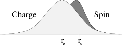
Figure 1: For a particle of finite extent the charge and spin distributions in real space are in general do not coincide. The same is true of the charge and spin distributions in reciprocal space.

II.4 Carrier spin, spin torque and consequences of finite particle size

The fact that carriers have a finite extent in real and wave-vector space has profound implications for particle dynamics and transport. These implications were pointed out in a previous publication Culcer using the semiclassical language of wave-packets and will be elaborated in this section from the density matrix point of view. For the sake of clarity we will specialize in spin, although the discussion in this section applies to any quantity.

When considering the transport of spin in a system composed of many carriers, one must associate a spin distribution with each individual carrier. A center of spin may be defined for each particle by ${\bf r}_{s}=\frac{\langle\hat{\bf r}\hat{s}\rangle}{\langle\hat{s}\rangle}$. This definition may be troublesome if the expectation value of the spin operator were zero, but its only purpose is to illustrate a physical principle. Evidently, if one replaced the spin operator with the charge or mass one would obtain the particle position as given by (9), which we will refer to as ${\bf r}_{c}$. It is obvious from the definition of ${\bf r}_{s}$ that in the general case there is no reason for the center of the spin distribution of an individual particle to be the same as the actual particle position. This center will be different for each component of the spin operator. Furthermore, since spin is not conserved in the presence of e.g. spin-orbit interactions, ${\bf r}_{s}$ may also be a function of time. This suggests that the spin distribution of one carrier will in general have a different shape than its charge distribution, and that the time development of the two distributions may be quite different. These facts are illustrated in Figs. 1 and 2.

To evaluate the average carrier spin consider the expectation value of the operator $\hat{s}$, which stands for any one component of the spin operator. The result is

$$\begin{split}{\rm Tr}\,\hat{\rho}\hat{s}={\rm tr}\int\,d{\cal V}\,\rho\,\bar{s},\end{split}$$ (22)

where $\bar{s}_{n^{\prime}n}=\langle\bar{u}_{n^{\prime}}|\hat{s}|\bar{u}_{n}\rangle$ are the matrix elements of the spin operator. In the presence of spin-orbit interactions a spin torque is associated with the spin of every carrier, which accounts for the non-conservation of spin, as shown in Fig. 2. The average carrier torque is found by evaluating the expectation value of $\hat{\tau}=\frac{i}{\hbar}[\tilde{H},\hat{s}]$. The result is

$$\begin{split}{\rm Tr}\,\hat{\rho}\hat{\tau}={\rm tr}\int\,d{\cal V}\,\rho\,\bar{\tau},\end{split}$$ (23)

where $\bar{\tau}_{n^{\prime}n}=\langle\bar{u}_{n^{\prime}}|\hat{\tau}|\bar{u}_{n}\rangle$.

As a result of the distinction between ${\bf r}_{s}$ and ${\bf r}_{c}$, in calculations of spin-related quantities which use the center of charge as the reference, multipole terms must be taken into account in addition to the average quantities calculated above. For example, in the distribution of spin a spin dipole will be present, as well as higher order multipole terms, which are assumed small. The spin dipole is found as the expectation value $\langle\hat{\bf r}\hat{s}\rangle$, evaluated in the appendix, and yields the gauge field

$$\bar{\bf M}^{s}_{n^{\prime}n}=\frac{i}{2}(\langle\bar{u}_{n^{\prime}}|\hat{s}|\frac{\partial\bar{u}_{n}}{\partial{\bf q}}\rangle-\langle\frac{\partial\bar{u}_{n^{\prime}}}{\partial{\bf q}}|\hat{s}|\bar{u}_{n}\rangle).$$ (24)

In contrast to ${\bf r}_{s}$, $\bar{\bf M}^{s}$ is well defined. Similarly, in the distribution of torque of an individual particle a torque dipole will be present. The torque gauge field $\bar{\bf M}^{\tau}=\langle\hat{\bf r}\hat{\tau}\rangle$ is given, as shown in the appendix, by

$$\bar{\bf M}^{\tau}_{n^{\prime}n}=\frac{i}{2}(\langle\bar{u}_{n^{\prime}}|\hat{\tau}|\frac{\partial\bar{u}_{n}}{\partial{\bf q}}\rangle-\langle\frac{\partial\bar{u}_{n^{\prime}}}{\partial{\bf q}}|\hat{\tau}|\bar{u}_{n}\rangle).$$ (25)

$\bar{\bf M}^{s}$ and $\bar{\bf M}^{\tau}$ are gauge dependent. It will prove useful to define gauge-covariant dipoles as $\bar{\bf p}^{s}=\bar{\bf M}^{s}-\frac{1}{2}\{\bar{\cal R},\bar{s}\}$ and $\bar{\bf p}^{\tau}=\bar{\bf M}^{\tau}-\frac{1}{2}\{\bar{\cal R},\bar{\tau}\}$ respectively. The remainder of the discussion of these gauge-covariant spin and torque dipoles is deferred to section IV.

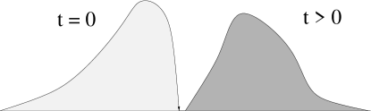
Figure 2: In the presence of spin-orbit interactions the spin distribution of a particle changes in time. The horizontal axis may represent position or wave vector.

II.5 Carrier spin velocity in an electric field

We define the spin velocity as the expectation value $\langle\hat{s}\hat{\bf v}\rangle$, where products of non-commuting operators are assumed to be symmetrized. The result is

$$\begin{split}{\rm Tr}\,\hat{\rho}\hat{s}\hat{\bf v}={\rm tr}\int\,d{\cal V}\,\rho\,\bar{\bf v}^{s}.\end{split}$$ (26)

The spin velocity $\bar{\bf v}^{s}$ is given by

$$\begin{array}[]{rl}\bar{\bf v}^{s}=&\displaystyle\frac{d}{dt}\langle\hat{\bf r}\hat{s}\rangle-\langle\hat{\bf r}\hat{\tau}\rangle\\[9.47217pt] =&\displaystyle\frac{d\bar{\bf M}^{s}}{dt}-\bar{\bf M}^{\tau}.\end{array}$$ (27)

In order to write the velocity in a gauge covariant form, we replace in the above $\bar{\bf M}^{s}=\bar{\bf p}^{s}+\frac{1}{2}\{\bar{\cal R},\bar{s}\}$ and $\bar{\bf M}^{\tau}=\bar{\bf p}^{\tau}+\frac{1}{2}\{\bar{\cal R},\bar{\tau}\}$. This yields immediately

$$\begin{split}\bar{\bf v}^{s}=\frac{1}{2}\{\frac{d\bar{\cal R}}{dt},\bar{s}\}+\frac{d\bar{\bf p}^{s}}{dt}-\bar{\bf p}^{\tau}.\end{split}$$ (28)

Equation (28) is the gauge-covariant form of equation (10) in Ref. [2], the integrand of which represents the spin velocity. The first term in (28)is a convective contribution and represents a moving electron transporting its average spin along with it. The second term is the time derivative of the spin dipole while the last term is the torque dipole which takes into account the non-conservation of spin. We may incorporate $\bar{\bf p}^{\tau}$ into a modified spin velocityCulcer ; Junren , which we shall call $\bar{\bf v}^{t}$, by $\bar{\bf v}^{t}=\bar{\bf v}^{s}+\bar{\bf p}^{\tau}$. The modified spin velocity is given simply by:

$$\begin{split}\bar{\bf v}^{t}=\frac{1}{2}\{\frac{d\bar{\cal R}}{dt},\bar{s}\}+\frac{d\bar{\bf p}^{s}}{dt}.\end{split}$$ (29)

The importance of this definition of the velocity will be seen in the following section, when the macroscopic spin current is introduced.

III Many particle distributions

We will consider the macroscopic distributions of charge and spin starting from the formalism we have developed. In particular, our discussion of the corrections to the spin density, current and torque distributions is motivated by the observation that the existing literature has omitted various contributions to spin transport. Several works have used semiclassical concepts but did not arrive at answers containing all the terms we have derived.

The particle number density is defined by the formula:

$$n({\bf R},t)={\rm Tr}[\hat{\rho}\delta({\bf R}-\hat{\bf r})].$$ (30)

The trace operation Tr involves integration over r. The procedure we follow has affinities with the coarse graining of electrodynamics in material media Jackson . The size of the carriers is taken to be smaller than the length scale of the Wigner function. We regard the $\delta$-function as a sampling functionJackson with a width somewhere between the microscopic scale of the carriers and the macroscopic scale of the Wigner function. The rationale for regarding the $\delta$-function as a sampling function comes from the realization that often the physics of the problem does not require absolute resolution of position, provided that the resolution is finer than the length scale of the external field. Since the variance of $\hat{\bf r}$ is finite, the $\delta$-function may be expanded in a Taylor series about the dummy variable r in the form $\delta({\bf R}-\hat{\bf r})=\delta({\bf R}-{\bf r})-\nabla_{\bf R}\cdot(\hat{\bf r}-{\bf r})\delta({\bf R}-{\bf r})+{\cal O}[(\hat{\bf r}-{\bf r})^{2}]$. The expansion is truncated at the first order for simplicity but we will show in the next section that all the terms may be recovered in a concise and elegant fashion. The number density can be expressed as:

$$n({\bf R},t)={\rm tr}\int d^{3}q\,(\rho-\nabla_{\bf R}\cdot\rho\,\bar{\mathcal{R}}).$$ (31)

In the above $\rho$ stands for $\rho({\bf q},{\bf R})$, an abbreviation which will be frequently used in the remainder of the article. Note that the gauge field $\bar{\cal R}$ in (31) plays the role of a dipole.

III.1 Electrical charge and current densities

The charge density is defined by the formula

$$n^{q}({\bf R},t)=q\,n({\bf R},t)=q\,{\rm Tr}[\hat{\rho}\delta({\bf R}-\hat{\bf r})].$$ (32)

The charge $q$ is not to be confused with the wave vector q. The charge current density ${\bf J}^{q}$ is defined by the equation

$${\bf J}^{q}({\bf R},t)=q\,{\rm Tr}[\hat{\rho}\delta({\bf R}-\hat{\bf r})\hat{\bf v}].$$ (33)

The charge equation of continuity in the absence of external sources and disorder,

$$\frac{\partial n^{q}}{\partial t}+\nabla\cdot{\bf J}^{q}=0,$$ (34)

is readily verified from the first-principles definitions of the charge and current densities.

When the $\delta$-function is expanded the current density takes the form

$${\bf J}^{q}({\bf R},t)=q\,{\rm tr}\int\frac{d^{3}q}{(2\pi)^{3}}\,\rho\,\bar{\bf v}.$$ (35)

The velocity matrix elements $\bar{\bf v}_{n^{\prime}n}=\langle\bar{u}_{n^{\prime}}|\tilde{\bf v}|\bar{u}_{n}\rangle$ as shown in the appendix, where $\tilde{\bf v}=e^{-i{\bf q}\cdot\hat{\bf r}}\hat{\bf v}e^{i{\bf q}\cdot\hat{\bf r}}$. Since in the equation of continuity it is the gradient of the current that appears, we have not included in (35) corrections to the current which arise from the fact that the velocity distribution of a single carrier is different from its charge distribution. These corrections are in principle present but have been omitted for simplicity.

In homogeneous systems the gradient term in (35) drops out of the equation of continuity and, based on equations (17) and (35), the charge current can be expressed as the time rate of change of the gauge field $\bar{\cal R}$

$${\bf J}^{q}({\bf R},t)=q\,{\rm tr}\int\frac{d^{3}q}{(2\pi)^{3}}\,\rho\,\frac{d\bar{\cal R}}{dt}.$$ (36)

III.2 Spin, spin current and spin torque densities

The spin density is defined as

$$S({\bf R},t)={\rm Tr}[\hat{\rho}\delta({\bf R}-\hat{\bf r})\hat{s}],$$ (37)

while the torque density takes the form

$${\cal T}({\bf R},t)={\rm Tr}[\hat{\rho}\delta({\bf R}-\hat{\bf r})\hat{\tau}]$$ (38)

and the spin current density is defined as

$${\bf J}^{s}({\bf R},t)={\rm Tr}[\hat{\rho}\delta({\bf R}-\hat{\bf r})\hat{s}\hat{\bf v}].$$ (39)

In the absence of disorder the spin equation of continuity is

$$\frac{\partial S}{\partial t}+\nabla\cdot{\bf J}^{s}={\cal T},$$ (40)

which is verified from the first-principles definitions introduced above.

The ${\delta}$-functions are expanded in the same way as for the particle number density, whereupon the spin density can be expressed as

$$S({\bf R},t)={\rm tr}\int\frac{d^{3}q}{(2\pi)^{3}}\,(\rho\,\bar{s}-\nabla_{\bf R}\cdot\rho\,\bar{\bf M}^{s}),$$ (41)

and the torque density is

$${\cal T}({\bf R},t)={\rm tr}\int\frac{d^{3}q}{(2\pi)^{3}}\,(\rho\,\bar{\tau}-\nabla_{\bf R}\cdot\rho\,\bar{\bf M}^{\tau}).$$ (42)

Ignoring the gradient term, the spin current is

$${\bf J}^{s}({\bf R},t)={\rm tr}\int\frac{d^{3}q}{(2\pi)^{3}}\,\rho\,\bar{\bf v}^{s}.$$ (43)

In analogy with the modified spin velocity of the previous section, a modified spin current ${\bf J}^{t}$ may be defined by:

$$\begin{array}[]{rl}{\bf J}^{t}({\bf R},t)=&\displaystyle{\rm tr}\int\frac{d^{3}q}{(2\pi)^{3}}\,\rho\,\bar{\bf v}^{t}\\[9.47217pt] =&\displaystyle{\rm tr}\int\frac{d^{3}q}{(2\pi)^{3}}\,\rho\,\left(\frac{1}{2}\{\frac{d\bar{\cal R}}{dt},\bar{s}\}+\frac{d\bar{\bf p}^{s}}{dt}\right).\end{array}$$ (44)

The equation of continuity satisfied by this current in the clean limit is:

$$\frac{\partial S}{\partial t}+\nabla\cdot{\bf J}^{t}={\rm tr}\int\frac{d^{3}q}{(2\pi)^{3}}\,\rho\,\bar{\tau}.$$ (45)

In many models, such as the spherical four-band Luttinger modelLuttinger , the RHS vanishes when all bands in the subspace are taken into account. In that case the spin current ${\bf J}^{t}$ is conserved. Much effort has been devoted to finding a conserved spin current. In our previous work Culcer ; Junren we have argued, based on semiclassical ideas, that the closest one can come to a conserved spin current is by including the torque dipole in the definition of the current. In this article we have derived this current from a density matrix point of view and show that it supports our earlier conclusions. To date, the definition ${\bf J}^{t}$ is the closest one has come to a conserved spin current. Moreover, as shown also by Zarea and Ulloa Zarea , the behavior of the modified spin current may be rather different from that of ${\bf J}^{s}$.

IV Gauge transformations

We have argued in section II that in discussing transport of an observable one must take into account the fact that the distribution of that observable for each individual carrier in general involves a dipole correction, and in principle also higher-order corrections. If the quantity being transported is not conserved then the determination of its rate of change also involves a dipole correction. The existence of what appears to be a sound physical argument for the inclusion of these corrections suggests that objects such as the spin dipole and the torque dipole are not simply mathematical artifacts meant to facilitate calculations. It is appropriate to investigate whether they are in fact fundamental quantities with a true physical meaning. If that were the case, they ought to be expressible in a gauge-covariant way and to give rise to observable effects.

In addition to these considerations, our aim of providing a physically transparent formalism requires a test of the gauge covariance of the macroscopic quantities and equations of motion we have derived in this article. The physics contained in them must be independent of the choice of basis functions. Furthermore, the physical discussion can become cluttered with futile and meaningless objects if it is formulated in terms of gauge-dependent objects. In contrast, the gauge-covariant expressions we derive below are simple, elegant and transparent.

A general local gauge transformation is represented by $|\bar{u}_{m}\rangle\rightarrow O_{mn}|\bar{u}_{n}\rangle$, with $O_{mn}=O_{mn}(\tilde{\bf q})$ and $m$ and $n$ are indices of bands in the subspace under consideration. Under this operation

$$\bar{\cal R}\rightarrow\tilde{\cal R}+i(O^{-1}\frac{\partial O}{\partial\tilde{\bf q}}),$$ (46)

in which $\tilde{\cal R}$ stands for $O\bar{\cal R}O^{-1}$. The Berry curvature for one band $\bar{\bf\Omega}_{n}$ is discussed extensively in the paper of Sundaram and NiuGanesh . One important additional detail which emerges from the transformation given by (46) and the definition $\bar{\bf\Omega}_{n}=\nabla_{\tilde{\bf q}}\times\bar{\cal R}_{n}$ is the fact that, if the curvature is non-zero, one cannot make a gauge transformation to eliminate $\bar{\cal R}_{n}$. It can be easily shown that, whereas $\bar{\cal R}_{n}$ is gauge dependent, the Berry curvature is gauge covariant. Therefore if $\bar{\bf\Omega}_{n}$ is non-zero in one gauge it is non-zero in all gauges and there is no gauge in which $\bar{\cal R}_{n}$ can be zero. As a result, in systems in which the curvature is non-zero the gauge-dependent position shift is necessarily present in the Wigner function. It can be regarded as a ‘penalty’ for working with the position operator in a basis of definite wave vector.

IV.1 Gauge covariance of macroscopic densities

The Wigner function itself changes under the gauge transformation defined above. Using (6), we find that, to first order in $O$, the Wigner function changes as

$$\rho\rightarrow\tilde{\rho}+\frac{i}{2}\nabla_{\bf R}\cdot\{\tilde{\rho},O^{-1}\frac{\partial O}{\partial\tilde{\bf q}}\},$$ (47)

where $\tilde{\rho}=O^{-1}\rho O$ (the opposite of the gauge connection $\bar{\cal R}$).

All the macroscopic densities defined in the previous sections are covariant under a local gauge transformation. This will be demonstrated for the spin density. Under the above gauge transformation, the gauge field $\bar{\bf M}^{s}$ transforms as

$$\begin{split}\bar{\bf M}^{s}\rightarrow\tilde{\bf M}^{s}+\frac{i}{2}\{{\tilde{s}},O^{-1}\frac{\partial O}{\partial\tilde{\bf q}}\}.\end{split}$$ (48)

The matrix elements of the transformed gauge field $\tilde{\bf M}^{s}$ are given by $\tilde{\bf M}^{s}_{n^{\prime}n}=\frac{i}{2}(\langle\bar{u}_{n^{\prime}}|\tilde{s}|\frac{\partial\bar{u}_{n}}{\partial\tilde{\bf q}}\rangle-\langle\frac{\partial\bar{u}_{n^{\prime}}}{\partial\tilde{\bf q}}|\tilde{s}|\bar{u}_{n}\rangle)$ and the transformed spin operator $\tilde{s}=O^{-1}\hat{s}O$. To first order the extra terms acquired by the spin density under a gauge transformation are

$${\rm tr}(\tilde{\rho}\{\tilde{s},O^{-1}\frac{\partial O}{\partial\tilde{\bf q}}\}-\{\tilde{\rho},O^{-1}\frac{\partial O}{\partial\tilde{\bf q}}\}\tilde{s})=0,$$ (49)

so that the spin density remains gauge covariant. The cancellation remains true for all orders in the expansion. Similarly, the charge and current densities do not acquire additional terms under the local gauge transformation introduced above. The extra terms appearing as a result of the transformation cancel when the trace is taken. When the change in the Wigner function under a gauge transformation is taken into account the overall expressions are gauge covariant.

IV.2 Gauge-covariant expressions for spin and torque dipoles

Equation (31) for the particle number density can be formally written the following way

$$n({\bf R},t)={\rm tr}\int d^{3}q\,\rho({\bf q},{\bf R}-\bar{\cal R}).$$ (50)

Re-expressing the integrand in this manner is tantamount to making, in the density matrix, the replacement $\rho({\bf q},{\bf r})\rightarrow\rho({\bf q},{\bf r}-\bar{\cal R})$. To ensure the gauge covariance of the number density the Fourier dual r is replaced by the true position ${\bf r}+\bar{\cal R}$, as illustrated in Fig. 3. This is the same position as found in section II. If the subspace contains one band expression (50) is an exact result, not simply a formal way of writing the number density.

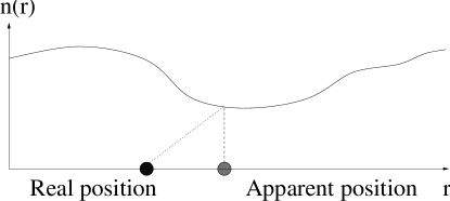
Figure 3: The position which appears in the Wigner function is not the real position.

Examining more closely the spin density as given in (41) it is evident that, whereas the spin density itself is gauge covariant, its individual constituents are not. If one were to consider the integrand of the dipole term in (41) without the Wigner function, this quantity would not by itself be gauge covariant. We have already constructed a gauge-covariant spin dipole $\bar{\bf p}^{s}=\bar{\bf M}^{s}-\frac{1}{2}\{\bar{\cal R},\bar{s}\}$. In terms of the gauge-covariant spin dipole, the spin density can be re-expressed as

$$\begin{split}S({\bf R},t)={\rm tr}\int\frac{d^{3}q}{(2\pi)^{3}}\,(\rho\,\bar{s}-\nabla_{\bf R}\cdot\rho\,\bar{\cal R}\,\bar{s}-\nabla_{\bf R}\cdot\rho\,\bar{\bf p}^{s}).\end{split}$$ (51)

It can be formally written the following way

$$S({\bf R},t)={\rm tr}\int\frac{d^{3}q}{(2\pi)^{3}}\,[\rho({\bf q},{\bf R}-\bar{\cal R})\,\bar{s}-\nabla_{\bf R}\cdot\rho({\bf q},{\bf R}-\bar{\cal R})\,\bar{\bf p}^{s}].$$ (52)

The gauge-covariant spin dipole $\bar{\bf p}^{s}$, as pointed out above, is the result of a carrier’s center of spin being different from its center of charge.

In the same way the gauge-covariant torque dipole has been defined by $\bar{\bf p}^{\tau}=\bar{\bf M}^{\tau}-\frac{1}{2}\{\bar{\cal R},\bar{\tau}\}$. Carrying out an identical manipulation to that for the spin density, use of the gauge-covariant torque dipole allows us to rewrite the torque density formally as

$${\cal T}({\bf R},t)={\rm tr}\int\frac{d^{3}q}{(2\pi)^{3}}\,[\rho({\bf q},{\bf R}-\bar{\cal R})\,\bar{\tau}-\nabla_{\bf R}\cdot\rho({\bf q},{\bf R}-\bar{\cal R})\,\bar{\bf p}^{\tau}].$$ (53)

A similar formal expression exists for the spin current. Evidently, since these expressions are simply a rewriting of the spin, torque and current densities, the equation of continuity satisfied by them is unaltered.

We remark that the gauge-covariant quantities introduced throughout this paper are well defined. In fact, even though the density matrix was expressed in a basis of extended Bloch states, by means of various manipulations we have been able to obtain well-defined formulas for all the objects relevant in transport.

Finally, as described by Dudarev et al. Artem in the context of atomic physics, optical lattices can be constructed which mimic the spin-orbit interaction. In such a lattice, a wave packet can be constructed using cold atoms and the evolution of its centers of mass and spin can be followed. In the same spirit, Kato et al. Kato have shown that it is possible to follow the motion of a spin packet in solid state systems, which demonstrates the feasibility of an analogous experiment in InGaAs. This would provide a way to measure a spin dipole directly.

V Summary

We have formulated a theory suitable for describing the dynamics of particles in both single and multiple bands. The one-band results known from the wave-packet formalism, including the terms connected to the Berry phase, emerge from our theory. The formalism can be applied to any clean system regardless of the dimensionality of the Hilbert space under consideration. As a result of the gauge degree of freedom of the basis functions, the position vector which is used as a label of the carrier must be modified by a gauge-dependent shift in order to obtain the true particle position. We have shown the way to define macroscopic density distributions for conserved and non-conserved operators. In the case of spin we have highlighted the correspondence between the multipole terms which appear in the density-matrix formalism and those found earlier in the wave-packet formalism and we have shown that experiments can be performed to identify the effect of a spin dipole.

DC was supported by the NSF under grant number DMR-0404252. QN was supported by the DOE under grant number DE-FG03-02ER45958.

VI Appendix

We will present in this appendix some of the proofs and evaluations which require lengthier calculations and would interrupt the flow if incorporated into the main text. For all derivations except the first, the $|\bar{u}_{m}\rangle$ and $|u_{m}\rangle$ are interchangeable.

VI.1 Proof of Eq. (14) for degenerate bands

The perturbed eigenfunctions are given by Eq.(14):

$$|\bar{u}_{m}\rangle=|u_{m}\rangle-\sum_{n\neq m}\frac{\langle u_{n}|i\hbar\frac{d}{dt}|u_{m}\rangle}{\varepsilon_{m}-\varepsilon_{n}}|u_{n}\rangle.$$

For a set of degenerate bands the equilibrium part of the density matrix is proportional to the identity matrix $I$ and will have the form $f_{0}\,I$, where $f_{0}$ is usually the Fermi-Dirac distribution. Transport theory often distinguishes between intrinsic effects, which are due to the equilibrium part of the density matrix, and extrinsic effects, which are due to the non-equilibrium correction to it. If we wish to evaluate the expectation value of an operator $\hat{A}$ using the equilibrium part of the density matrix for a set of degenerate bands, which for simplicity here we will take as being two dimensional, the following quantity must be evaluated:

$$\langle\hat{A}\rangle=f_{0}(\langle\bar{u}_{1}|\hat{A}|\bar{u}_{1}\rangle+\langle\bar{u}_{2}|\hat{A}|\bar{u}_{2}\rangle)$$

The perturbed wave functions are given by:

$$\begin{array}[]{rl}&\displaystyle|\bar{u}_{1}\rangle=|u_{1}\rangle-\frac{\langle u_{2}|i\hbar\frac{d}{dt}|u_{1}\rangle}{\varepsilon_{1}-\varepsilon_{2}}|u_{2}\rangle-\sum_{n\neq 1,2}\frac{\langle u_{n}|i\hbar\frac{d}{dt}|u_{1}\rangle}{\varepsilon_{m}-\varepsilon_{n}}|u_{n}\rangle\\[9.47217pt] &\displaystyle|\bar{u}_{2}\rangle=|u_{2}\rangle-\frac{\langle u_{1}|i\hbar\frac{d}{dt}|u_{2}\rangle}{\varepsilon_{2}-\varepsilon_{1}}|u_{1}\rangle-\sum_{n\neq 1,2}\frac{\langle u_{n}|i\hbar\frac{d}{dt}|u_{m}\rangle}{\varepsilon_{m}-\varepsilon_{n}}|u_{n}\rangle.\end{array}$$

The expectation values are:

$$\begin{array}[]{rl}&\displaystyle\langle\bar{u}_{1}|\hat{A}|\bar{u}_{1}\rangle=A_{11}-\frac{\langle u_{1}|i\hbar\frac{du_{2}}{dt}\rangle}{\varepsilon_{1}-\varepsilon_{2}}A_{21}-\frac{\langle u_{2}|i\hbar\frac{du_{1}}{dt}\rangle}{\varepsilon_{1}-\varepsilon_{2}}A_{12}+\sum_{1}^{out}\\[9.47217pt] &\displaystyle\langle\bar{u}_{2}|\hat{A}|\bar{u}_{2}\rangle=A_{22}-\frac{\langle u_{1}|i\hbar\frac{du_{2}}{dt}\rangle}{\varepsilon_{2}-\varepsilon_{1}}A_{21}-\frac{\langle u_{2}|i\hbar\frac{du_{1}}{dt}\rangle}{\varepsilon_{2}-\varepsilon_{1}}A_{12}+\sum_{2}^{out}.\end{array}$$

In the above $\sum_{1}^{out}$ and $\sum_{2}^{out}$ stand for the sums involving the bands outside the degenerate manifold and $A_{ij}=\langle u_{i}|\hat{A}|u_{j}\rangle$. The denominators of the terms involving $A_{12}$ and $A_{21}$ have opposite signs. Therefore, adding up the expectation values we obtain:

$$(\langle\bar{u}_{1}|\hat{A}|\bar{u}_{1}\rangle+\langle\bar{u}_{2}|\hat{A}|\bar{u}_{2}\rangle)=A_{11}+A_{22}+\sum_{1}^{out}+\sum_{2}^{out}.$$

Therefore the terms with diverging denominators cancel out.

VI.2 Evaluation of position matrix elements

In the general case, the expectation value of the position operator is given by

$$\begin{split}\langle\hat{\bf r}\rangle=\int d{\cal V}\,\rho_{nn^{\prime}}\int d^{3}Q\,e^{-i{\bf Q}\cdot{\bf r}}\langle\bar{u}_{n^{\prime}-}|\hat{\bf r}e^{i{\bf Q}\cdot\hat{\bf r}}|\bar{u}_{n+}\rangle\\ =\int d{\cal V}\,\rho_{nn^{\prime}}\int d^{3}Q\,e^{-i{\bf Q}\cdot{\bf r}}\langle\bar{u}_{n^{\prime}-}|(-i\frac{\partial}{\partial{\bf Q}}e^{i{\bf Q}\cdot\hat{\bf r}})|\bar{u}_{n+}\rangle.\end{split}$$

We can expand the integrand in the above equation and obtain

$$\begin{array}[]{rl}\langle\bar{u}_{n^{\prime}-}|\hat{\bf r}e^{i{\bf Q}\cdot\hat{\bf r}}|\bar{u}_{n+}\rangle=&\displaystyle-i\frac{\partial}{\partial{\bf Q}}\langle\bar{u}_{n^{\prime}-}|e^{i{\bf Q}\cdot\hat{\bf r}}|\bar{u}_{n+}\rangle\\[9.47217pt] &\displaystyle+\langle i\frac{\partial\bar{u}_{n^{\prime}-}}{\partial{\bf Q}}|e^{i{\bf Q}\cdot\hat{\bf r}}|\bar{u}_{n+}\rangle\\[9.47217pt] &\displaystyle+\langle\bar{u}_{n^{\prime}-}|e^{i{\bf Q}\cdot\hat{\bf r}}|i\frac{\partial\bar{u}_{n+}}{\partial{\bf Q}}\rangle\\[9.47217pt] &\displaystyle+{\bf r}\langle\bar{u}_{n^{\prime}-}|e^{i{\bf Q}\cdot\hat{\bf r}}|\bar{u}_{n+}\rangle.\end{array}$$

All four brackets represent integrals of products of lattice periodic functions and exponentials. They will all eventually be proportional to $\delta({\bf Q})$. Because of this fact the first term above integrates to zero. The partial derivatives in the second and third terms are evaluated by expanding the lattice periodic Bloch wave functions about q, treating Q as a small parameter

$$\begin{split}|\bar{u}_{n+}\rangle=|\bar{u}_{n\tilde{\bf q}}\rangle+\frac{{\bf Q}}{2}\cdot|\frac{\partial\bar{u}_{n\tilde{\bf q}}}{\partial\tilde{\bf q}}\rangle\\ |\bar{u}_{n-}\rangle=|\bar{u}_{n\tilde{\bf q}}\rangle-\frac{{\bf Q}}{2}\cdot|\frac{\partial\bar{u}_{n\tilde{\bf q}}}{\partial\tilde{\bf q}}\rangle\end{split}$$ (54)

In the limit in which ${\bf Q}\rightarrow 0$

$$|\frac{\partial\bar{u}_{n\pm}}{\partial{\bf Q}}\rangle=\pm\frac{1}{2}|\frac{\partial\bar{u}_{n\tilde{\bf q}}}{\partial\tilde{\bf q}}\rangle.$$

Consequently

$$\langle\bar{u}_{n^{\prime}-}|\hat{\bf r}e^{i{\bf Q}\cdot\hat{\bf r}}|\bar{u}_{n+}\rangle={\bf r}\delta_{n^{\prime}n}+\bar{\cal R}_{n^{\prime}n},$$

and the expectation value of the position vector yields, finally

$$\begin{split}\langle\hat{\bf r}\rangle=\int d{\cal V}\,\rho_{nn^{\prime}}({\bf r}\delta_{n^{\prime}n}+\bar{\cal R}_{n^{\prime}n}).\end{split}$$

VI.3 Evaluation of spin and torque gauge fields

The spin gauge field is found in an analogous fashion to the expectation value of the position operator

$$\begin{split}\langle\hat{\bf r}\hat{s}\rangle=\int d{\cal V}\,\rho_{nn^{\prime}}\int d^{3}Q\,e^{-i{\bf Q}\cdot{\bf r}}\langle\bar{u}_{n^{\prime}-}|\hat{\bf r}\hat{s}e^{i{\bf Q}\cdot\hat{\bf r}}|\bar{u}_{n+}\rangle\\ =\int d{\cal V}\,\rho_{nn^{\prime}}\int d^{3}Q\,e^{-i{\bf Q}\cdot{\bf r}}\langle\bar{u}_{n^{\prime}-}|\hat{s}(-i\frac{\partial}{\partial{\bf Q}}e^{i{\bf Q}\cdot\hat{\bf r}})|\bar{u}_{n+}\rangle\\ =\int d{\cal V}\,\rho_{nn^{\prime}}\bar{\bf M}^{s}_{n^{\prime}n}.\end{split}$$

Expanding the above,

$$\begin{array}[]{rl}\langle\bar{u}_{n^{\prime}-}|\hat{\bf r}\hat{s}e^{i{\bf Q}\cdot\hat{\bf r}}|\bar{u}_{n+}\rangle=&\displaystyle-i\frac{\partial}{\partial{\bf Q}}\langle\bar{u}_{n^{\prime}-}|\hat{s}e^{i{\bf Q}\cdot\hat{\bf r}}|\bar{u}_{n+}\rangle\\[9.47217pt] &\displaystyle+\langle i\frac{\partial\bar{u}_{n^{\prime}-}}{\partial{\bf Q}}|\hat{s}e^{i{\bf Q}\cdot\hat{\bf r}}|\bar{u}_{n+}\rangle\\[9.47217pt] &\displaystyle+\langle\bar{u}_{n^{\prime}-}|\hat{s}e^{i{\bf Q}\cdot\hat{\bf r}}|i\frac{\partial\bar{u}_{n+}}{\partial{\bf Q}}\rangle.\end{array}$$

Using the same arguments as in the previous section, the first term integrates to zero, and after evaluating the brackets involving the exponential and the lattice-periodic functions, we obtain in the limit ${\bf Q}\rightarrow 0$

$$\bar{\bf M}^{s}_{n^{\prime}n}=\frac{i}{2}(\langle\bar{u}_{n^{\prime}}|\hat{s}|\frac{\partial\bar{u}_{n}}{\partial{\bf q}}\rangle-\langle\frac{\partial\bar{u}_{n^{\prime}}}{\partial{\bf q}}|\hat{s}|\bar{u}_{n}\rangle).$$ (55)

An almost identical derivation applies for the expectation value $\langle\hat{\bf r}\hat{\tau}\rangle\equiv\frac{1}{2}\langle\{\hat{\bf r},\hat{\tau}\}\rangle$. The only difference is that, since $\hat{\tau}$ may be a function of wave vector, an additional term involving $-i\frac{\partial\hat{\tau}}{\partial{\bf Q}}$ is generated. However, that term drops out when the anti-commutator is taken, leaving us with the result

$$\bar{\bf M}^{\tau}_{n^{\prime}n}=\frac{i}{2}(\langle\bar{u}_{n^{\prime}}|\hat{\tau}|\frac{\partial\bar{u}_{n}}{\partial{\bf q}}\rangle-\langle\frac{\partial\bar{u}_{n^{\prime}}}{\partial{\bf q}}|\hat{\tau}|\bar{u}_{n}\rangle).$$ (56)

VI.4 Finite variance of carrier position

Since the expectation value of the carrier position has been shown above to contain no divergences, if the expectation value $\langle\hat{\bf r}^{2}\rangle$ is not divergent then the variance $\langle\hat{\bf r}^{2}\rangle-\langle\hat{\bf r}\rangle^{2}$ is also finite. To see that the variance of the particle position does not contain any divergences, we need to evaluate the expectation value $\langle\hat{\bf r}^{2}\rangle$. This requires us to evaluate the matrix element

$$\begin{split}\langle\bar{u}_{n^{\prime}-}|\hat{r}^{2}e^{i{\bf Q}\cdot\hat{\bf r}}|\bar{u}_{n+}\rangle=-\langle\bar{u}_{n^{\prime}-}|(\frac{\partial^{2}}{\partial Q^{2}}e^{i{\bf Q}\cdot\hat{\bf r}})|\bar{u}_{n+}\rangle.\end{split}$$

First note that an expression of the form $-A\frac{\partial^{2}B}{\partial Q^{2}}CD$ can be written as

$$\begin{array}[]{rl}-A\frac{\partial^{2}B}{\partial Q^{2}}CD=&\displaystyle-\frac{\partial^{2}}{\partial Q^{2}}(ABCD)\\[9.47217pt] &\displaystyle+2\frac{\partial}{\partial{\bf Q}}\cdot[\frac{\partial A}{\partial{\bf Q}}BCD+AB\frac{\partial}{\partial{\bf Q}}(CD)]\\[9.47217pt] &\displaystyle-\frac{\partial^{2}A}{\partial Q^{2}}BCD-2\frac{\partial A}{\partial{\bf Q}}\cdot B\frac{\partial}{\partial{\bf Q}}(CD)\\[9.47217pt] &\displaystyle-AB\frac{\partial^{2}B}{\partial Q^{2}}(CD).\end{array}$$

In the case we are considering, all the products involve brackets which are proportional to $\delta({\bf Q})$. As a result, all the terms on the first line vanish under integration with respect to Q and only the terms on the second line need to be evaluated. Writing them out explicitly,

$$\begin{array}[]{rl}&\displaystyle\langle\bar{u}_{n^{\prime}-}|\hat{r}^{2}e^{i{\bf Q}\cdot\hat{\bf r}}|\bar{u}_{n+}\rangle=r^{2}\langle\bar{u}_{n^{\prime}-}|e^{i{\bf Q}\cdot\hat{\bf r}}|\bar{u}_{n+}\rangle)\\[9.47217pt] &\displaystyle-\langle\frac{\partial^{2}\bar{u}_{n^{\prime}-}}{\partial Q^{2}}|e^{i{\bf Q}\cdot\hat{\bf r}}|\bar{u}_{n+}\rangle-\langle\bar{u}_{n^{\prime}-}|e^{i{\bf Q}\cdot\hat{\bf r}}|\frac{\partial^{2}\bar{u}_{n+}}{\partial Q^{2}}\rangle\\[9.47217pt] &\displaystyle+2i{\bf r}\cdot(\langle\frac{\partial\bar{u}_{n^{\prime}-}}{\partial{\bf Q}}|e^{i{\bf Q}\cdot\hat{\bf r}}|\bar{u}_{n+}\rangle+\langle\bar{u}_{n^{\prime}-}|e^{i{\bf Q}\cdot\hat{\bf r}}|\frac{\partial\bar{u}_{n+}}{\partial{\bf Q}}\rangle)\\[9.47217pt] &\displaystyle-2\langle\frac{\partial\bar{u}_{n^{\prime}-}}{\partial{\bf Q}}|e^{i{\bf Q}\cdot\hat{\bf r}}|\frac{\partial\bar{u}_{n+}}{\partial{\bf Q}}\rangle.\end{array}$$

In order to evaluate the differentials, the wave functions are expanded as in (54) except that now the expansion must be made to second order in Q. The final result is

$$\begin{array}[]{rl}\langle\hat{\bf r}^{2}\rangle=&\displaystyle\int d{\cal V}\,\rho_{nn^{\prime}}[r^{2}\delta_{n^{\prime}n}+2{\bf r}\cdot\bar{\cal R}_{n^{\prime}n}\\[9.47217pt] &\displaystyle+\frac{1}{2}\langle\frac{\partial\bar{u}_{n^{\prime}}}{\partial\tilde{\bf q}}|\cdot|\frac{\partial\bar{u}_{n}}{\partial\tilde{\bf q}}\rangle-\frac{1}{4}(\langle\frac{\partial^{2}\bar{u}_{n^{\prime}}}{\partial\tilde{q}^{2}}|\bar{u}_{n}\rangle\\[9.47217pt] &\displaystyle+\langle\bar{u}_{n^{\prime}}|\frac{\partial^{2}\bar{u}_{n}}{\partial\tilde{q}^{2}}\rangle)].\end{array}$$

This is clearly finite so the variance of the position operator is finite.

VI.5 Evaluation of velocity matrix elements

The velocity matrix element $\langle\bar{u}_{n^{\prime}-}|e^{-i{\bf q}_{-}\cdot\hat{\bf r}}\hat{\bf v}e^{i{\bf q}_{+}\cdot\hat{\bf r}}|\bar{u}_{n+}\rangle$ is easily evaluated as

$$\begin{array}[]{rl}&\displaystyle\langle\bar{u}_{n^{\prime}-}|e^{-i{\bf q}_{-}\cdot\hat{\bf r}}\hat{\bf v}e^{i{\bf q}_{+}\cdot\hat{\bf r}}|\bar{u}_{n+}\rangle\\[9.47217pt] &\displaystyle=\int d^{3}r^{\prime}\,\bar{u}_{n^{\prime}-}({\bf r}^{\prime})e^{-i{\bf q}_{-}\cdot{\bf r}^{\prime}}\hat{\bf v}e^{i{\bf q}_{+}\cdot{\bf r}^{\prime}}\bar{u}_{n+}({\bf r}^{\prime})\\[9.47217pt] &\displaystyle=\int d^{3}r^{\prime}\,e^{i{\bf Q}\cdot{\bf r}^{\prime}}\bar{u}_{n^{\prime}-}({\bf r}^{\prime})(e^{-i{\bf q}_{+}\cdot\hat{\bf r}^{\prime}}\hat{\bf v}e^{i{\bf q}_{+}\cdot\hat{\bf r}^{\prime}})\bar{u}_{n+}({\bf r}^{\prime})\\[9.47217pt] &\displaystyle=\delta({\bf Q})\int d^{3}r^{\prime}\,\bar{u}_{n^{\prime}}({\bf r}^{\prime})\tilde{\bf v}\bar{u}_{n}({\bf r}^{\prime})=\delta({\bf Q})\langle\bar{u}_{n^{\prime}}|\tilde{\bf v}|\bar{u}_{n}\rangle.\end{array}$$

In the above we have abbreviated $\tilde{\bf v}=e^{-i{\bf q}\cdot\hat{\bf r}^{\prime}}\hat{\bf v}e^{i{\bf q}\cdot\hat{\bf r}^{\prime}}$.

We also need to evaluate the commutator $\frac{1}{2}\langle\bar{u}_{n^{\prime}-}|e^{-i{\bf q}_{-}\cdot(\hat{\bf r}-{\bf r})}\{\hat{\bf v},(\hat{\bf r}-{\bf r})\}e^{i{\bf q}_{+}\cdot(\hat{\bf r}-{\bf r})}|\bar{u}_{n+}\rangle$. One half of the commutator is evaluated as

$$\begin{array}[]{rl}&\displaystyle\langle\bar{u}_{n^{\prime}-}|e^{-i{\bf q}_{-}\cdot(\hat{\bf r}-{\bf r})}\hat{\bf v}(\hat{\bf r}-{\bf r})e^{i{\bf q}_{+}\cdot(\hat{\bf r}-{\bf r})}|\bar{u}_{n+}\rangle\\[9.47217pt] &\displaystyle=\langle\bar{u}_{n^{\prime}-}|e^{-i{\bf q}_{-}\cdot(\hat{\bf r}-{\bf r})}\hat{\bf v}[-i\frac{\partial}{\partial{\bf q}_{+}}e^{i{\bf q}_{+}\cdot(\hat{\bf r}-{\bf r})}]|\bar{u}_{n+}\rangle\\[9.47217pt] &\displaystyle=-i\frac{\partial}{\partial{\bf q}_{+}}\langle\bar{u}_{n^{\prime}-}|e^{-i{\bf q}_{-}\cdot(\hat{\bf r}-{\bf r})}\hat{\bf v}e^{i{\bf q}_{+}\cdot(\hat{\bf r}-{\bf r})}|\bar{u}_{n+}\rangle\\[9.47217pt] &\displaystyle+\langle\bar{u}_{n^{\prime}-}|e^{-i{\bf q}_{-}\cdot(\hat{\bf r}-{\bf r})}\frac{\partial\hat{\bf v}}{\partial{\bf q}_{+}}e^{i{\bf q}_{+}\cdot(\hat{\bf r}-{\bf r})}|\bar{u}_{n+}\rangle\\[9.47217pt] &\displaystyle+\langle\bar{u}_{n^{\prime}-}|e^{-i{\bf q}_{-}\cdot(\hat{\bf r}-{\bf r})}\hat{\bf v}e^{i{\bf q}_{+}\cdot(\hat{\bf r}-{\bf r})}|i\frac{\partial\bar{u}_{n+}}{\partial{\bf q}_{+}}\rangle,\end{array}$$

while the other is

$$\begin{array}[]{rl}&\displaystyle\langle\bar{u}_{n^{\prime}-}|e^{-i{\bf q}_{-}\cdot(\hat{\bf r}-{\bf r})}(\hat{\bf r}-{\bf r})\hat{\bf v}e^{i{\bf q}_{+}\cdot(\hat{\bf r}-{\bf r})}|\bar{u}_{n+}\rangle\\[9.47217pt] &\displaystyle=\langle\bar{u}_{n^{\prime}-}|[i\frac{\partial}{\partial{\bf q}_{-}}e^{-i{\bf q}_{-}\cdot(\hat{\bf r}-{\bf r})}]\hat{\bf v}e^{i{\bf q}_{+}\cdot(\hat{\bf r}-{\bf r})}|\bar{u}_{n+}\rangle\\[9.47217pt] &\displaystyle=i\frac{\partial}{\partial{\bf q}_{-}}\langle\bar{u}_{n^{\prime}-}|e^{-i{\bf q}_{-}\cdot(\hat{\bf r}-{\bf r})}\hat{\bf v}e^{i{\bf q}_{+}\cdot(\hat{\bf r}-{\bf r})}|\bar{u}_{n+}\rangle\\[9.47217pt] &\displaystyle-\langle i\frac{\partial\bar{u}_{n-}}{\partial{\bf q}_{-}}|e^{-i{\bf q}_{-}\cdot(\hat{\bf r}-{\bf r})}\hat{\bf v}e^{i{\bf q}_{+}\cdot(\hat{\bf r}-{\bf r})}|\bar{u}_{n^{\prime}+}\rangle\\[9.47217pt] &\displaystyle-\langle\bar{u}_{n^{\prime}-}|e^{-i{\bf q}_{-}\cdot(\hat{\bf r}-{\bf r})}\frac{\partial\hat{\bf v}}{\partial{\bf q}_{-}}e^{i{\bf q}_{+}\cdot(\hat{\bf r}-{\bf r})}|\bar{u}_{n+}\rangle.\end{array}$$

All the brackets in the above two equations are proportional to $\delta({\bf Q})$, causing most of the terms to cancel. We are left with:

$$\begin{split}\frac{1}{2}\langle\bar{u}_{n^{\prime}-}|e^{-i{\bf q}_{-}\cdot(\hat{\bf r}-{\bf r})}\{\tilde{\bf v},(\hat{\bf r}-{\bf r})\}e^{i{\bf q}_{+}\cdot(\hat{\bf r}-{\bf r})}|\bar{u}_{n+}\rangle\\ =\frac{i}{2}\delta({\bf Q})(\langle\bar{u}_{n}|\tilde{\bf v}|\frac{\partial\bar{u}_{n^{\prime}}}{\partial{\bf q}}\rangle-\langle\frac{\partial\bar{u}_{n}}{\partial{\bf q}}|\tilde{\bf v}|\bar{u}_{n^{\prime}}\rangle).\end{split}$$

VI.6 Effect of gauge transformation on $\rho({\bf q},{\bf r})$

The operator $\hat{\rho}$ must be invariant under gauge transformations. From the expansion of the density operator in Bloch eigenstates,

$$\hat{\rho}=\sum_{n,n^{\prime}}\sum_{{\bf k},{\bf k}^{\prime}}\rho_{nn^{\prime}}({\bf k},{\bf k}^{\prime})|\bar{\psi}_{n\tilde{\bf k}}\rangle\langle\bar{\psi}_{n^{\prime}\tilde{\bf k}^{\prime}}|,$$

it is evident that, if the wave functions change according to $|\bar{\psi}_{m\tilde{\bf k}}\rangle\rightarrow O_{mn}(\tilde{\bf k})|\bar{\psi}_{n\tilde{\bf k}}\rangle$, then $\rho_{nn^{\prime}}({\bf k},{\bf k}^{\prime})$ must transform to $O^{-1}\rho O$. Using the definition of $\rho_{nn^{\prime}}({\bf k},{\bf k}^{\prime})$ in terms of the Wigner function,

$$\rho({\bf q},{\bf r})=\int\frac{d^{3}Q}{(2\pi)^{3}}\,e^{i{\bf Q}\cdot{\bf r}}\rho({\bf q}_{+},{\bf q}_{-}),$$

and remembering that ${\bf k}\equiv{\bf q}_{+}$ and ${\bf k}^{\prime}\equiv{\bf q}_{-}$, we obtain

$$\rho({\bf q},{\bf r})\rightarrow\int\!\frac{d^{3}Q}{(2\pi)^{3}}e^{i{\bf Q}\cdot{\bf r}}O^{-1}(\tilde{\bf q}_{+})\rho({\bf q}_{+},{\bf q}_{-})O(\tilde{\bf q}_{-}).$$

The matrices $O^{-1}(\tilde{\bf q}_{+})$ and $O(\tilde{\bf q}_{-})$ may be expanded about their arguments as:

$$\begin{array}[]{rl}&\displaystyle O^{-1}(\tilde{\bf q}_{+})=O^{-1}(\tilde{\bf q})+\frac{{\bf Q}}{2}\cdot\frac{\partial O^{-1}(\tilde{\bf q})}{\partial\tilde{\bf q}}+O(Q^{2})\\[9.47217pt] &\displaystyle O(\tilde{\bf q}_{-})=O(\tilde{\bf q})-\frac{{\bf Q}}{2}\cdot\frac{\partial O(\tilde{\bf q})}{\partial\tilde{\bf q}}+O(Q^{2}).\end{array}$$

Then, to first order in ${\bf Q}$, abbreviating $O(\tilde{\bf q})$ to $O$ and $\rho({\bf q}_{+},{\bf q}_{-})$ to $\rho_{q}$,

$$\begin{array}[]{rl}&\displaystyle O^{-1}(\tilde{\bf q}_{+})\rho_{q}({\bf q}_{+},{\bf q}_{-})O(\tilde{\bf q}_{-})\\[9.47217pt] &\displaystyle=O^{-1}\rho_{q}O+\frac{{\bf Q}}{2}\cdot(\frac{\partial O^{-1}}{\partial\tilde{\bf q}}\rho_{q}O-O^{-1}\rho_{q}\frac{\partial O}{\partial\tilde{\bf q}})\\[9.47217pt] &\displaystyle=\tilde{\rho}_{q}+\frac{{\bf Q}}{2}\cdot(\frac{\partial O^{-1}}{\partial\tilde{\bf q}}O\tilde{\rho}_{q}-\tilde{\rho}_{q}O^{-1}\frac{\partial O}{\partial\tilde{\bf q}}),\end{array}$$

where $\tilde{\rho}_{q}=O^{-1}\rho_{q}O$. The last line is obtained by inserting $OO^{-1}$ or $O^{-1}O$ as appropriate. Since $\frac{\partial}{\partial\tilde{\bf q}}(OO^{-1})=0$, we have $\frac{\partial O^{-1}}{\partial\tilde{\bf q}}O=-O^{-1}\frac{\partial O}{\partial\tilde{\bf q}}$ and

$$\begin{split}\rho\rightarrow\tilde{\rho}-\frac{{\bf Q}}{2}\cdot\{\tilde{\rho},O^{-1}\frac{\partial O}{\partial\tilde{\bf q}}\}.\end{split}$$

Finally, writing $-\frac{{\bf Q}}{2}=\frac{i}{2}\nabla_{\bf r}e^{i{\bf Q}\cdot{\bf r}}$, we recover formula (47) for the transformation of $\rho({\bf q},{\bf r})$.

References

• (1) N. W. Ashcroft and N. D. Mermin, Solid State Physics, 2nd edition (Saunders College Publishing, New York, 1976).
• (2) D. Culcer, J. Sinova, N. A. Sinitsyn, T. Jungwirth, A. H. MacDonald, and Q. Niu, Phys. Rev. Lett. 93, 046602 (2004).
• (3) D. Culcer, Y. G. Yao, A. H. MacDonald, and Q. Niu, Phys. Rev. B (2005).
• (4) J. Sinova, D. Culcer, Q. Niu, N. A. Sinitsyn, T. Jungwirth, and A. H. MacDonald, Phys. Rev. Lett. 92, 126603 (2004).
• (5) S. Murakami, N. Nagaosa, and S.-C. Zhang, Science 301, 1348 (2003).
• (6) S. Murakami, N. Nagaosa, and S.-C. Zhang, Phys. Rev. B 69, 235206 (2004).
• (7) S. Zhang, Phys. Rev. Lett 85, 393 (2000).
• (8) S. Zhang and Z. Yang, Phys. Rev. Lett. 94, 066602 (2005).
• (9) L. Hu, J. Gao, and S. Q. Shen, Phys. Rev. B 70, 235323 (2004).
• (10) J. Inoue, G.W.Bauer, L. W. Molenkamp, Phys. Rev. B 67, 033104 (2003).
• (11) E. G. Mishchenko, A. V. Shytov, and B. I. Halperin, Phys. Rev. Lett. 93, 226602 (2004).
• (12) O. V. Dimitrova, Phys. Rev. B 71, 245327 (2005).
• (13) G. Y. Guo, Y. Yao, and Q. Niu, Phys. Rev. Lett. 94, 226601 (2005).
• (14) Y. Yao and Z. Fang, cond-mat/0502351.
• (15) J. Callaway, Quantum Theory of the Solid State (Academic Press, New York, 1976).
• (16) G. Sundaram and Q. Niu, Phys. Rev. B 59, 14915 (1999).
• (17) M. V. Berry, Proc. R. Soc. London Ser. A, 392, 45 (1984).
• (18) D. Culcer, A. H. MacDonald, and Q. Niu, Phys. Rev. B 68, 045327 (2003).
• (19) T. Jungwirth, Q. Niu, and A. H. MacDonald, Phys. Rev. Lett. 88, 207208 (2002).
• (20) Yugui Yao, Leonard Kleinman, A. H. MacDonald, Jairo Sinova, T. Jungwirth, Ding-sheng Wang, Enge Wang, and Qian Niu, Phys. Rev. Lett. 92, 037204 (2004).
• (21) D. Culcer, Y. G. Yao, and Q. Niu, Phys. Rev. B (2005).
• (22) R. Shindou and K. Imura, Nucl. Phys. B 720 [FS], 399 (2005).
• (23) S. A. Wolf, D. D. Awschalom, R. A. Buhrman, J. M. Daughton, S. von Molnar, M. L. Roukes, A. Y. Chtchelkanova, and D. M. Treger , Science 294, 1488 (2001).
• (24) P.R. Hammar and M. Johnson, Phys. Rev. Lett. 88, 066806 (2002).
• (25) Y. K. Kato, R. C. Myers, A. C. Gossard, and D. D. Awschalom, Science 306, 1910 (2004).
• (26) J. Wunderlich, B. Kaestner, J. Sinova, and T. Jungwirth, Phys. Rev. Lett. 94, 047204 (2005).
• (27) Y. Kato, R. C. Myers, A. C. Gossard, and D. D. Awschalom, Phys. Rev. Lett. 93, 176601 (2004).
• (28) L. E. Reichl, A Modern Course in Statistical Physics (University of Texas Press, Austin, 1980).
• (29) An interesting recent article, G. A. Fiete and E. G. Heller, Phys. Rev. A 68, 022112 (2003), discusses this topic from a somewhat different point of view.
• (30) R. G. Littlejohn and W. G. Flynn, Phys. Rev. A 44, 5239 (1991).
• (31) M. Marder, Condensed Matter Physics (John Wiley, New York, 2000).
• (32) M.I. Dyakonov and V. I. Perel, JETP Lett. 35A, 459 (1971).
• (33) M.I. Dyakonov and V. I. Perel, Sov. Phys. JETP 33, 1053 (1971).
• (34) M.I. Dyakonov and V. I. Perel, Sov. Phys. Solid State 13, 3023 (1972).
• (35) M.I. Dyakonov and V. Y. Kachorovskii, Sov. Phys. Semicond. 20, 110 (1986).
• (36) E. L. Ivchenko, Y. B. Lyanda-Geller, and G. E. Pikus, Sov. Phys. JETP 71, 550 (1990).
• (37) G. E. Pikus and A. N. Titkov in Optical Orientation (Elsevier Science Publications, Amsterdam, 1984).
• (38) A. G. Aronov, Yu. B. Lyanda-Geller, and G. E. Pikus, Sov. Phys. JETP 73, 537 (1991).
• (39) Y. Qi and S. Zhang, Phys. Rev. B 65, 214407 (2002), ibid. 67, 052407 (2003).
• (40) U. Fano, Rev. Mod. Phys. 29, 74 (1957).
• (41) A. Messiah, Quantum Mechanics (Dover Publications, New York, 2000).
• (42) Ping Zhang, Junren Shi, Di Xiao, and Qian Niu, Phys. Rev. Lett 96, 076604 (2006).
• (43) J.D. Jackson, Classical Electrodynamics, 3rd edition (John Wiley $\&$ Sons, 1999), section 6.6 (pp. 248-258).
• (44) J. M. Luttinger, Phys. Rev. 102, 1030 (1956).
• (45) M. Zarea and S. E. Ulloa, Phys. Rev. B 73, 165306 (2006).
• (46) A. M. Dudarev, R. B. Diener, I. Carusotto, and Q. Niu Phys. Rev. Lett. 92, 153005 (2004)
• (47) Y. Kato et al., Nature 427, 50 (2004).