Switchable resonant coupling of flux qubits

Abstract

We propose a coupling scheme, where two or more flux qubits with different eigenfrequencies share Josephson junctions with a coupler loop devoid of its own quantum dynamics. Switchable two-qubit coupling is realized by tuning the frequency of the AC magnetic flux through the coupler to a combination frequency of two of the qubits. The coupling allows any or all of the qubits to be simultaneously at the degeneracy point and can change sign.

I Introduction

The scheme by Makhlin et al.Makhlin et al. (1999) for coupling superconducting qubits was recently followed by several proposals for tunable couplingYou et al. (202, 2003); Filippov et al. (2003); Averin and Bruder (2003); Kim and Hong (2004); Plourde et al. (2004); Castellano et al. (2005); Maassen van den Brink et al. (2005) between superconducting qubits.You and Nori (2005) Broadly speaking, these approaches couple qubits through the exchange of virtual excitations in the coupler circuit, in which the energy separation $E_{0}$ between the ground and first excited state is much larger than the tunnel splitting $\Delta$ in the qubits. The coupling strength $J$ is controlled by tuning the energy of the coupling circuit, via a magnetic field (if the coupler is a SQUID), or via a gate voltage (if it is a Cooper pair box).

In principle, the above approaches provide a DC coupling between qubits, and they allow the realization of entangling gates only if the difference $|\Delta_{a}-\Delta_{b}|$ between the tunnel splittings of the corresponding qubits is smaller than the coupling energy $J$.

In the opposite limit, when $|\Delta_{a}-\Delta_{b}|\gg|J|$, it was shownLiu et al. (2006) that the qubit-qubit interaction can be controlled by an external variable-frequency magnetic field at the combination frequencies, $|\Delta_{a}\pm\Delta_{b}|/\hbar$. This approachLiu et al. (2006) (coupling by using a time-dependent magnetic flux, or TDMF) is advantageous due to the resonant character of the coupling: in experiments it is often easier to produce fast and precise frequency shifts of the RF control signal, as opposed to changes in the amplitude of the DC signal. The proposal in Ref. Liu et al., 2006 also did not require additional, dedicated coupler circuits. Its disadvantage was that at least one of the qubits must be biased away from the optimal point, which could make its operation more difficult and reduce its decoherence time.

Later on, a combination of the TDMF approach with a dedicated coupler circuit led to tunable-coupling proposals in Refs. Bertet et al., 2006 and Niskanen et al., 2006, where both coupled qubits could be simultaneously at their optimal points.

In this paper we propose an alternative realization of the TDMF coupling, which allows to switch the coupling on and off, and to change its sign. Our proposal has an advantage over both the approaches of Refs. Liu et al., 2006; Bertet et al., 2006; Niskanen et al., 2006, and the generalization of Ref. Niskanen et al., 2006 to the Josephson coupling (described in Section V of this paper), in simultaneously providing: (1) a coupling for arbitrarily biased qubits, (2) a higher coupling energy, (3) enhanced protection from the flux noise, and (4) the elimination of the parasitic first-order DC coupling.

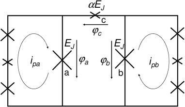
Figure 1: Schematic diagram of two flux qubits and the three-junction coupler circuit.

II Model

In our proposal, the coupling circuit is a small-inductance superconducting loop ($L_{c}\rightarrow 0$) with three Josephson junctions (denoted by a, b, c in Fig. 1). The shared junctions a, b ensure a significantly stronger qubit-loop coupling than in the case of purely inductive (like in Refs. Bertet et al., 2006; Niskanen et al., 2006) or galvanic connection.Plourde et al. (2004) A controllable DC coupling in a similar device has been recently proposed and realized experimentally,Kim and Hong (2004); Maassen van den Brink ; van der Ploeg et al. with the coupling energy $J_{\rm DC}=1.7$ GHz.

For the sake of simplicity, and without loss of generality, we assume that the junctions $a$ and $b$ have the same Josephson energy $E_{J}=\Phi_{0}I_{c}/2\pi$. The qubit-qubit coupling is realized by the (small) junction $c$, with the Josephson energy $\alpha E_{J}\ll E_{J}$. The coupler circuit ($a$, $b$, and $c$) has a high plasma frequency, $\omega_{p}\sim\sqrt{8E_{J}E_{C}}/\hbar$, so that its energy-level separation is much larger than all relevant characteristic energies ($J$ and $\Delta_{a,b}$) of the system. The large Josephson energy and large capacitances ($C\gg C_{c}\approx\alpha C$) of the coupling junctions ensure that $E_{C}/E_{J}\ll 1$. This allows us to neglect their degrees of freedom and to consider them as passive elements, which convert the bias currents $I_{pa}$ and $I_{pb}$, produced by the persistent currents circulating in the attached flux qubits, into the phase shift, and therefore the energy shift, of the small Josephson junction $c$.

III Coupling strength

Let us now concentrate on the coupler circuit. The action of the two flux qubits on it can be represented by the bias currents through the junctions $a$ and $b$. (Due to the dominance of the Josephson coupling, we can disregard the geometric mutual inductances between them.) The qubit-qubit interaction energy is obtained by taking into account the total potential energy. The latter is the free energy of the coupler plus the work performed by the qubits $a,b$ on the coupler circuit to keep their persistent currents constant.Likharev (1984) By making use of the quantization condition for the gauge-invariant phase differences, $\varphi_{a}-\varphi_{b}+\varphi_{c}=-2\pi\Phi_{c}/\Phi_{0}$, where $\Phi_{c}$ is the magnetic flux through the coupler loop and $\Phi_{0}$ is the magnetic flux quantum, the reduced total energy $U_{t}$ can be written as

$$\tilde{U}_{t}\>\equiv\>U_{t}/E_{J}\>=-\cos\varphi_{a}-\cos\varphi_{b}$$

$$-\alpha\cos(2\pi f_{c}+\varphi_{a}-\varphi_{b})-i_{pa}\,\varphi_{a}+i_{pb}\,\varphi_{b},$$ (1)

where $f_{c}=\Phi_{c}/\Phi_{0}$, $i_{pa}=I_{pa}/I_{c}$, and $i_{pb}=I_{pb}/I_{c}$. For small values of $\alpha,$ $i_{pa},$ and $i_{pb}$, this potential forms a well with a minimum near the point $(\varphi_{a},\varphi_{b})=(0,0)$. This is the Hamiltonian of a three-junction flux qubitOrlando et al. (1999) with biased junctions, which can be reduced to the Hamiltonian of a perturbed two-dimensional oscillator

$$H = \frac{\hat{P}_{+}^{2}}{2M_{+}}+\frac{\hat{P}_{-}^{2}}{2M_{-}}+E_{J}\varphi_{+}^{2}+\kappa E_{J}(\varphi_{-}-\varphi_{-}^{*})^{2}$$ (2)

$$+ E_{J}[\varphi_{+}(i_{pb}-i_{pa})-\varphi_{-}(i_{pa}+i_{pb})].$$

Here $\varphi_{\pm}=(\varphi_{a}\pm\varphi_{b})/2$, $\hat{P}_{\pm}=i\hbar\partial/\partial\varphi_{\pm}$, $M_{+}=2C(\Phi_{0}/2\pi)^{2}$, $M_{-}=M_{+}(1+2\alpha)$, $\kappa=1+2\alpha\cos(2\pi f_{c}+2\varphi_{-}^{*})$, and $\varphi_{-}^{*}=-\alpha\sin(2\pi f_{c})/(1+2\alpha\cos(2\pi f_{c}))$. (see Ref. Orlando et al., 1999 for details). The perturbation is $E_{J}[\varphi_{+}(i_{pb}-i_{pa})-\varphi_{-}(i_{pa}+i_{pb})]$.

From Eq. (2), the normal frequencies of the coupler are $\omega_{+}=\sqrt{2E_{J}/M_{+}}$ and $\omega_{-}=\sqrt{2\kappa E_{J}/M_{-}}$. Its eigenstates, in the lowest order in $i_{pa},$ $i_{pb}$, are products $\Psi_{+,m}(\varphi_{+})\Psi_{-,n}(\varphi_{-})$ of the eigenstates of the normal modes. The first-order correction to the ground state energy of the coupler is zero, and the coupling energy is determined by the second-order correction:

$$E_{0}^{(2)} = \frac{E_{J}^{2}(i_{pa}+i_{pb})^{2}}{\hbar\omega_{-}}\left|\langle\Psi_{-,1}|\varphi_{-}|\Psi_{-,0}\rangle\right|^{2}$$ (3)

$$+ \frac{E_{J}^{2}(i_{pa}-i_{pb})^{2}}{\hbar\omega_{+}}\left|\langle\Psi_{+,1}|\varphi_{+}|\Psi_{+,0}\rangle\right|^{2}.$$

Thus, it is evident that the coupling is provided by the virtual photon exchange between the qubits and the coupler.

Separating the term proportional to $i_{pa}i_{pb}$ in the second-order correction in Eq. (3), we obtain the coupling energy

$$J=\frac{\kappa-1}{\kappa}E_{J}\frac{i_{pa}i_{pb}}{2}.$$ (4)

Inserting the definition of $\kappa$ into Eq. 4 the coupling energy of the three-junction coupler reads

$$J=\frac{\alpha E_{J}\;\cos(2\pi f_{c}\;+\;2\varphi_{-}^{*})}{1+2\alpha\cos(2\pi f_{c}\;+\;2\varphi_{-}^{*})}\;i_{pa}i_{pb}.$$ (5)

This expression obviously corresponds to the $\sigma_{z}\sigma_{z}$ coupling in the natural basis of qubit states (see, e.g., Eqs. (1,3) in Ref. van der Ploeg et al., )

$$H_{\rm int}(t)=J(f_{c})\,\sigma^{z}_{a}\,\sigma^{z}_{b}.$$ (6)

Obviously, the coupling (6) allows either one or both qubits to be in their optimal points. In the experiment in Ref. van der Ploeg et al., such interaction was used to realize a tunable DC coupling between qubits $a$ and $b$, by changing the coupler bias $f_{c}$. The strength and sign of the coupling depend on the precise value of $f_{c}$. As mentioned above, for time-domain operations it is often easier to manipulate the frequency of the AC signal $f_{c}(t)$, rather than the amplitude of a DC pulse. We will therefore use the TDMF approach initially proposed in Ref.Liu et al., 2006.

IV Effective coupling under TDMF

Let us first consider the effective coupling for an arbitrary $J(f_{c})$. Assuming the harmonic flux dependence,

$$f_{c}(t)=\nu_{0}+\nu_{1}\cos\Omega t,$$

for the reduced flux in the coupler circuit, and expanding $J(f_{c})$ near $\nu_{0}$, we reduce the Hamiltonian of the system to

$$H(t) = H_{0}+H_{1}=$$

$$- \frac{1}{2}\sum_{s=a,b}\Delta_{s}\sigma^{x}_{s}+\left(J_{\rm DC}(\nu_{0})+J^{\prime}(\nu_{0})\nu_{1}\cos\Omega t\right)\sigma^{z}_{a}\sigma^{z}_{b},$$

where $J^{\prime}(\nu_{0})$ is the first derivative of the coupling energy, taken at $\nu_{0}$. In the interaction representation this becomes

$$\tilde{H}(t)=H_{0}+\tilde{H}_{1}(t)$$ (8)

with

$$\tilde{H}_{1}=\left[J_{\rm DC}(\nu_{0})+(J^{\prime}(\nu_{0})\nu_{1}\cos\Omega t)\right](\sigma^{z}_{a}\cos\Delta_{a}t-\sigma^{y}_{a}\sin\Delta_{a}t)(\sigma^{z}_{b}\cos\Delta_{b}t-\sigma^{y}_{b}\sin\Delta_{b}t).$$ (9)

Assuming $\Delta_{a}-\Delta_{b}>0$ and $\Omega\approx\Delta_{a}\mp\Delta_{b}$, we see that (after averaging over the fast oscillations) only the coupling

$$H_{\rm eff}=\frac{J_{\rm AC}}{4}\left[\sigma^{z}_{a}\sigma^{z}_{b}\pm\sigma^{y}_{a}\sigma^{y}_{b}\right]$$ (10)

survives, where

$$J_{\rm AC}=J^{\prime}(\nu_{0})\nu_{1}.$$ (11)

The operator in the square brackets,

$$\sigma^{z}_{a}\,\sigma^{z}_{b}\pm\sigma^{y}_{a}\,\sigma^{y}_{b}\>=\>\left(\begin{array}[]{rrrr}1&0&0&-1\\ 0&-1&\pm 1&0\\ 0&\pm 1&-1&0\\ -1&0&0&1\end{array}\right),$$ (16)

is entangling and therefore can be used to construct universal quantum ciruits.Zhang et al. (2003)

Our results are somewhat similar to those of Ref. Niskanen et al., 2006. Let us describe the differences. Due to the Josephson, rather than inductive, coupling, our approach realizes larger coupling energies, therefore it allows smaller values of the parameter $\alpha$ and, correspondingly, is less nonlinear. For example, at $\alpha=0.01$ and $\nu_{0}=0.25$ the DC coupling $J_{\rm DC}(0.25)$ is close to zero and the AC coupling (Eq. (11)) $J^{\prime}(0.25)=2\pi E_{jc}i_{a}i_{b}$ is at a maximum (Fig. 2a). Using the experimental value of the DC coupling energy for the device shown in Fig. 1, $J_{0}(0)=1.7$ GHz,van der Ploeg et al. we find the AC coupling energy $J_{\rm AC}=10^{-2}J^{\prime}(0.25)\approx 100$ MHz (for the reduced magnetic flux amplitude $\nu_{1}=10^{-2}$). The DC and AC couplings can be increased by moving to the highly nonlinear regime with larger $\alpha>10^{-1}$, but now the points, corresponding to “zero” DC coupling and maximal AC coupling, do not coincide (Fig. 2b).

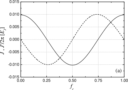
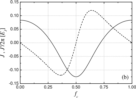
Figure 2: Coupling energy $J$ (solid line) and its first derivative $J^{\prime}$ (dashed line) as a function of the reduced applied magnetic flux $f_{c}$ through the coupler loop, for two parameters $\alpha=0.01$ (a) and $\alpha=0.1$ (b). The $J^{\prime}$ is scaled by a factor $2\pi$. When the nonlinear response of the coupler increases, the points of “zero” DC coupling and maximal AC coupling diverge from the common point $f_{c}=0.25$.

V Time-dependent magnetic flux coupling using an itermediary “qubit”

Now let us substitute the smaller junction by three Josephson junctions with sizes much smaller than the size of the coupling junctions $a,b$ (see Fig. 3). This is a generalized model of Ref. Niskanen et al., 2006, with the inductive coupling replaced by the stronger Josephson one. This allows to increase $\Delta_{c}$ and decrease the area of the qubits, improving the protection of the system against magnetic flux noise. Nevertheless we will see that this scheme is at a serious disadvantage compared to the coupling of Fig. 1, because it leads to a strong DC coupling between the qubits (i.e., parasitic DC coupling).

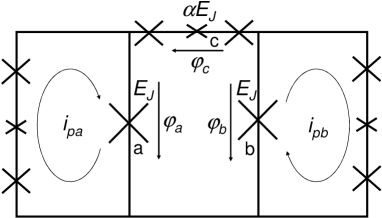
Figure 3: Schematic diagram of two flux qubits and the five-junction (“qubit”) coupler circuit.

We can now apply the same approach as in Eq.(3). The harmonic approximation of (2) is now invalid. Instead, the coupling energy is determined by the change of the ground state energy of the coupling “qubit” $c$,

$$\varepsilon(\varphi_{c})=-\frac{1}{2}\sqrt{[2E_{Jc}(\varphi_{c}-\pi)]^{2}+\Delta_{c}^{2}}.$$

Here $E_{Jc}=\Phi_{0}I_{pc}/2\pi$ and $\varphi_{c}$ is the phase difference across the “qubit” $c$. Expanding $\varepsilon(2\pi f_{c}+2\varphi_{-})$ at $2\pi f_{c}$ to second order, we obtain the potential of a two-dimensional linear harmonic oscillator with a new value of the constant

$$\kappa=1+2\left(\frac{\partial^{2}\tilde{\varepsilon}}{\partial\varphi^{2}_{c}}\right),$$

where $\tilde{\varepsilon}=\varepsilon/E_{J}$ is the normalized “qubit” energy. Substituting the new $\kappa$ in Eq. (4), we arrive at an expression for the coupling energy in the simple form

$$J = \frac{\partial^{2}\varepsilon}{\partial\varphi_{c}^{2}}\;i_{pa}i_{pb}$$

$$= \frac{\Delta_{c}}{8\pi^{2}}\left(\frac{2I_{pc}\Phi_{0}}{\Delta_{c}}\right)^{2}\left(1+\left(\frac{2I_{pc}\Phi_{0}}{\Delta_{c}}\tilde{f_{c}}\right)^{2}\right)^{-3/2}i_{qa}i_{qb},$$

where $\tilde{f_{c}}=f_{c}-0.5$. The derivative, $J^{\prime}=\partial J/\partial\tilde{f_{c}}$ has a maximum at $\tilde{f}_{\rm cm}=\Delta_{c}/4I_{pc}\Phi_{0}$:

$$J^{\prime}_{\rm max}\approx J_{\rm DC}(f_{cm})\>\left(\frac{2I_{pc}\Phi_{0}}{\Delta_{c}}\right).$$ (18)

Near this point, the AC coupling energy depends on the external magnetic flux only in the second order. This formula is equivalent to the expression (25) in Ref. Niskanen et al., 2006 provided that we use the standard normalization for currentsLikharev (1984) $i_{pa}=2\pi M_{ac}I_{pa}/\Phi_{0}$, $i_{pb}=2\pi M_{bc}I_{pb}/\Phi_{0}$ and neglect the mutual inductance between qubits. It is evident from Eq. (18) that the DC coupling cannot be tuned to zero without switching off the AC coupling, and it turns out to be much stronger than the latter. This is what we refer to as parasitic DC coupling. Because of large nonlinearity, the AC magnetic flux should be much smaller than $\Delta_{c}/2I_{pc}\Phi_{0}$. Taking, e.g., $\nu_{1}=10^{-2}\Delta_{c}/2I_{pc}\Phi_{0}$, the AC coupling energy becomes

$$J_{\rm AC}=J^{\prime}_{\rm max}\;\nu_{1}=10^{-2}J(f_{\rm cm}),$$ (19)

i.e., $J_{\rm AC}=10^{-2}J_{\rm DC}.$ More importantly, in our proposal the DC coupling can be switched off completely, and the AC coupling (100 MHz) is five times stronger than in Ref. Niskanen et al., 2006.

VI Conclusions

We propose a feasible switchable coupling between superconducting flux qubits, controlled by the resonant RF signal. Due to the frequency control, it is particularly suitable for time-domain operations with flux qubits. The coupling energy 100 MHz can be achieved by applying a magnetic flux $10^{-2}\Phi_{0}$ to the coupler with the combination frequency

$$\omega_{0}=|\Delta_{a}\pm\Delta_{b}|/\hbar.$$

The Josephson coupling allows to minimize the area of the devices, thus limiting the effects of the flux noise, and the coupler thus can act in an almost linear regime, which, in particular, suppresses the parasitic DC coupling. The resulting interaction term also acts as an entangling gate and enables the realization of a universal quantum circuit.