The two-site Bose–Hubbard model

Abstract

The two-site Bose–Hubbard model is a simple model used to study Josephson tunneling between two Bose–Einstein condensates. In this work we give an overview of some mathematical aspects of this model. Using a classical analysis, we study the equations of motion and the level curves of the Hamiltonian. Then, the quantum dynamics of the model is investigated using direct diagonalisation of the Hamiltonian. In both of these analyses, the existence of a threshold coupling between a delocalised and a self-trapped phase is evident, in qualitative agreement with experiments. We end with a discussion of the exact solvability of the model via the algebraic Bethe ansatz.

PACS: 03.75.Lm, 32.80.Pj, 03.75.Kk

This work is dedicated to the memory of Daniel Arnaudon

1 Introduction

The phenomenon of Bose–Einstein condensation, while predicted long ago [1, 2], is nowadays responsible for many current perspectives on the potential applications of quantum behaviour in mesoscopic systems. This point of view has arisen with the experimental observation of condensation in systems of ultracold dilute alkali gases, realised by several research groups using magnetic traps with various kinds of confining geometries [3, 4]. These types of experimental apparatus open up the possibility for studying quantum effects, such as Josephson tunneling and self-trapping [5, 6], in a macroscopic setting.

From the theoretical point of view, the two-site Bose–Hubbard model (see eq. (1) below), also known as the canonical Josephson Hamiltonian [7], has been a useful model in understanding tunneling phenomena. The simplicity of the model means that it is amenable to detailed mathematical analysis, as we will discuss below. However despite this apparent simplicity, the Hamiltonian captures the essence of competing linear and non-linear interactions, leading to interesting, non-trivial behaviour.

The Hamiltonian is given by

$$H = \frac{k}{8}(N_{1}-N_{2})^{2}-\frac{\Delta\mu}{2}(N_{1}-N_{2})-\frac{\cal{E}_{J}}{2}(b_{1}^{\dagger}b_{2}+b_{2}^{\dagger}b_{1}).$$ (1)

where $b_{1}^{\dagger},b_{2}^{\dagger}$ denote the single-particle creation operators in the two wells and $N_{1}=b_{1}^{\dagger}b_{1},N_{2}=b_{2}^{\dagger}b_{2}$ are the corresponding boson number operators. The total boson number $N_{1}+N_{2}$ is conserved and set to the fixed value of $N$. The coupling $k$ provides the strength of the scattering interaction between bosons, $\Delta\mu$ is the external potential and ${\cal E}_{J}$ is the coupling for the tunneling. The change ${\cal E}_{J}\rightarrow-{\cal E}_{J}$ corresponds to the unitary transformation $b_{1}\rightarrow b_{1},\,b_{2}\rightarrow-b_{2}$, while $\Delta\mu\rightarrow-\Delta\mu$ corresponds to $b_{1}\leftrightarrow b_{2}$. Therefore we will restrict our analysis to the case of ${\cal E}_{J},\,\Delta\mu\geq 0$. For $k>0$, following [7] it is useful to divide the parameter space into three regimes; viz. Rabi ($k/{\cal E}_{J}<<N^{-1}$), Josephson ($N^{-1}<<k/{\cal E}_{J}<<N$) and Fock ($N<<k/{\cal E}_{J}$). For these three regimes, there is a correspondence between (1) and the motion of a pendulum [7]. In the Rabi and Josephson regimes this motion is semiclassical, in contrast to the Fock regime. For both the Fock and Josephson regimes the analogy corresponds to a pendulum with fixed length, while in the Rabi regime the length varies.

In the present work, we give an overview of some of the mathematical aspects of (1). We undertake an analysis of the classical and the quantum dynamics of the system, and discuss how the system exhibits a threshold coupling, originally identified in [8], about which the dynamics abruptly changes. Below this threshold point the dynamics is delocalised, while above it the dynamics turns out to be localised (macroscopic self-trapping). This can be seen at both the classical and quantum level. The result is in qualitative agreement with experimental results [6]. We conclude by giving an outline of the algebraic Bethe ansatz solution of (1).

2 Classical dynamics

First we study a classical analogue of the model. Let $N_{j},\,\theta_{j},\,j=1,\,2$ be quantum variables satisfying the canonical relations

$$[\theta_{1},\,\theta_{2}]=[N_{1},\,N_{2}]=0,~{}~{}~{}~{}~{}[N_{j},\,\theta_{k}]=i\delta_{jk}I.$$

Using the fact that

$$\exp(i\theta_{j})N_{j}=(N_{j}+1)\exp(i\theta_{j})$$

we make a change of variables from the operators $b_{j},\,b_{j}^{\dagger},\,j=1,\,2$ via

$$b_{j}=\exp(i\theta_{j})\sqrt{N_{j}},~{}~{}~{}b_{j}^{\dagger}=\sqrt{N_{j}}\exp(-i\theta_{j})$$

such that the Heisenberg canonical commutation relations are preserved. Now define the variables

$$z=(N_{1}-N_{2})/N$$

$$\phi=N(\phi_{1}-\phi_{2})/2$$

where $z$ represents the fractional occupation difference (or the imbalance) and $\phi$ the phase difference. In the classical limit where $N$ is large, but still finite, we may equivalently consider the Hamiltonian [9, 10]

$$H(z,\phi)=\frac{{\cal E}_{J}N}{2}\left(\frac{\lambda}{2}z^{2}-\beta z-\sqrt{1-z^{2}}\cos({2\phi}/{N})\right)$$ (2)

where

$$\lambda=\frac{kN}{2{\cal E}_{J}},~{}~{}~{}~{}~{}\beta=\frac{\Delta\mu}{{\cal E}_{J}}$$

and $(z,\,\phi)$ are canonically conjugate variables. We note the Hamiltonian (2) obeys the symmetries

$$\left.H\left(z,\phi\right)\right|_{\lambda,\beta} = -\left.H\left(z,\phi+N\pi/2\right)\right|_{-\lambda,-\beta}$$

$$\left.H\left(z,\phi\right)\right|_{\lambda,\beta} = \left.H\left(-z,\phi\right)\right|_{\lambda,-\beta}.$$ (3)

The classical dynamics is given by Hamilton’s equations of motion

$$\dot{\phi} = \frac{\partial H}{\partial z}=\frac{{\cal E}_{J}N}{2}\left(\lambda z-\beta+\frac{z}{\sqrt{1-z^{2}}}\cos({2\phi}/{N})\right)$$

$$\dot{z} = -\frac{\partial H}{\partial\phi}=-{\cal E}_{J}\left(\sqrt{1-z^{2}}\sin({2\phi}/{N})\right).$$ (4)

Now we study the fixed points of the Hamiltonian (2), determined by the condition $\dot{z}=\dot{\phi}=0$. This leads to the following classification:

• $\phi=0$ and $z$ is a solution of

  $$\lambda z-\beta=-\frac{z}{\sqrt{1-z^{2}}}$$ (5)

  which has a unique real solution for $\lambda>0$.

• $\phi={N\pi}/{2}$ and $z$ is a solution of

  $$\lambda z-\beta=\frac{z}{\sqrt{1-z^{2}}}.$$ (6)

  This equation has either one, two or three real solutions for $\lambda>0$.
  

From eq. (6) we can determine that there are fixed point bifurcations for certain choices of the coupling parameters. These bifurcations allow us to divide the coupling parameter space in two regions. Setting $f(z)=\lambda z-\beta$ and $g(z)=z({1-z^{2}})^{-1/2}$, the boundary between the regions occurs when $f(z)$ is the tangent line to $g(z)$ at some value $z_{0}$. A standard analysis shows this occurs when $\lambda=g^{\prime}(z_{0})=(1-z_{0}^{2})^{-3/2}$. Requiring $f(z_{0})=g(z_{0})$ then yields the following relationship

$$\lambda=(1+\left|\beta\right|^{2/3})^{3/2}$$ (7)

determining the boundary. This is depicted in Fig. 1.

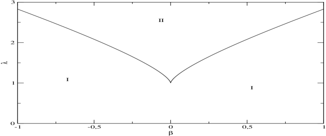
Figure 1: Coupling parameter space diagram identifying the different types of solutions for equation (6). In region I there is just one solution for $z$, a local maximum. In region II there are three solutions for $z$, two local maxima and a saddle point. The boundary separating regions I and II is given by (7).

This leads us to the following classification:

• $0<\lambda<1$: For any value of $\beta$ there is just one real solution, for which the Hamiltonian attains a local maximum.
  

• $\lambda>1$: Here transition couplings $\pm\beta_{0}$ appear, which can be seen from Fig. 1. For $\beta\in(-\beta_{0},\beta_{0})$, the equation has two locally maximal fixed points and one saddle point, while for $\beta>\beta_{0}$ or $\beta<-\beta_{0}$ the equation has just one real solution, a locally maximal fixed point.

We remark that in the absence of the external potential $(\Delta\mu=\beta=0)$ the transition value is given by $\lambda_{0}=1$. Using the symmetry relation (3) we can deduce that for the attractive case $\lambda<0$, $\lambda_{0}=-1$ is the coupling marking a bifurcation between a locally minimal fixed point (for $\lambda>-1$) and two locally minimal fixed points and a saddle point (for $\lambda<-1$). This is a supercritical pitchfork bifurcation of the classical ground state. The results of [14] predict that the ground-state entanglement, as measured by the von Neumann entropy, is maximal at this coupling. The numerical results of [15] confirm this.

Next we look at the dynamical evolution. In that which follows we will consider the equations (4) in the absence of the external field ($\Delta\mu=0$ or, equivalently, $\beta=0$). An analysis including the effect of this term can be found in references [11, 12]. We integrate (4) to find the time evolution for the imbalance $z$, using the initial condition $z(0)=1,\,\phi(0)=0$. By plotting $z$ against the time, it is evident that there is a threshold coupling $\lambda_{c}=2$ separating two different behaviours in the classical dynamics, as can be seen in Fig. 2:

• For $\lambda<2$ the system oscillates between $z=-1$ and $z=1$. Here the evolution is delocalised;

• For $\lambda>2$ the system oscillates between $z=0$ and $z=1$. Here the evolution is localised.

The threshold occuring at $\lambda_{c}=2$ was first observed in [8].

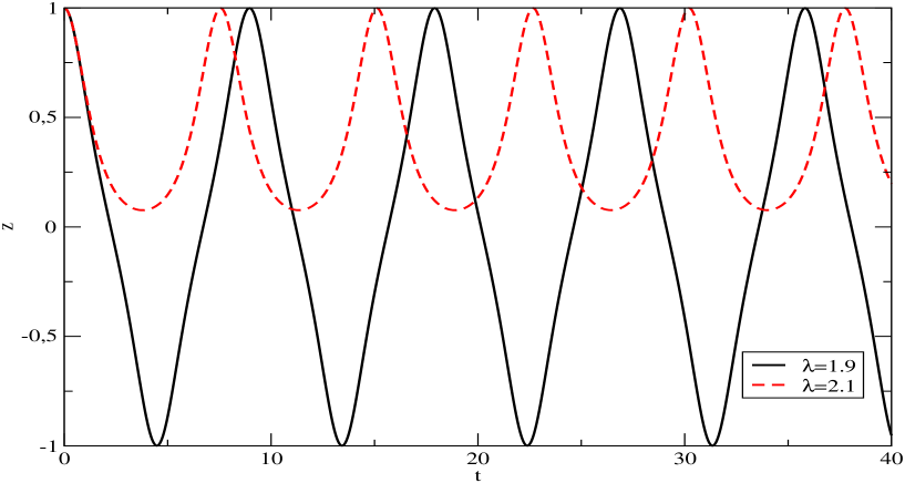
Figure 2: Time evolution for the imbalance $z$. The solid line is for $\lambda=1.9$, while the dashed curve is for $\lambda=2.1$. Here we are using $N=100$, ${\cal E}_{J}=1$ and the initial conditions $z(0)=1$, $\phi(0)=0$. The threshold coupling occurs at $\lambda_{c}=2$.

To help visualise the classical dynamics, it is useful to plot the level curves (constant energy curves) of the Hamiltonian (2) in phase space. Given an initial condition $(z(0),\phi(0))$, the system follows a trajectory along the level curve $H(z(0),\phi(0))$. In Fig. 3 we plot the level curves for different values of $\lambda$ ($\lambda=1.5$ on the left and $\lambda=2.5$ on the right), where we take $2\phi/N\in[-\pi,\,\pi]$. We can observe clearly two distinct scenarios:

• $\lambda>2$: Here we see that for the orbit with initial condition $z_{0}=1,\,\phi(0)=0$, $\phi$ increases monotonically (running phase mode). The evolution of $z$ is bounded in the interval $[0,1]$, leading to localisation (self-trapping).

• $\lambda<2$: Here we see that for the orbit with initial condition $z(0)=1,\,\phi(0)=0$, the evolution of $\phi$ is oscillatory and bounded in the interval $(-N\pi/2,\,N\pi/2)$. The evolution of $z$ is not bounded, leading to delocalisation.

(a)	(b)

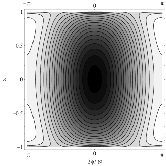
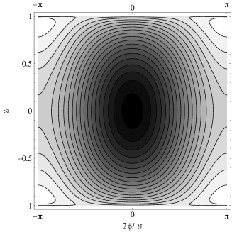
Figure 3: Level curves of the Hamiltonian (2) (a) for $\lambda=1.5$ (below the threshold point) and (b) for $\lambda=2.5$ (above the threshold point). We are using $N=100$ and ${\cal E}_{J}=1$. Above the threshold coupling running phase modes occur leading to localised evolution of $z$. Below the threshold coupling the evolution of $z$ is delocalised.

The threshold coupling $\lambda_{c}=2$ (or $k/{\cal E}_{\mathcal{J}}=4/N$, in terms of the original variables) separates two distinct dynamical behaviours. This value for the threshold between delocalisation and self-trapping also occurs for the quantum dynamics, as we will show in the next section.

3 Quantum dynamics

We will investigate the quantum dynamics of the Hamiltonian in the absence of the external potential $(\Delta\mu=0$) using the exact diagonalisation method. It is well known that the time evolution of any state is determined by $|\Psi(t)\rangle=U(t)|\phi_{0}\rangle$, where $U$ is the temporal evolution operator given by $U(t)=\sum_{m=0}^{M}|m\rangle\langle m|\exp(-iE_{m}t)$, $|m\rangle$ is an eigenstate with energy $E_{m}$ and $|\phi_{0}\rangle$ represents the initial state. Using these expressions we can compute the expectation value of the relative number of particles

$$\langle(N_{1}-N_{2})(t)\rangle=\langle\Psi(t)|N_{1}-N_{2}|\Psi(t)\rangle.$$ (8)

From Fig. 4 it is seen that the qualitative behaviour in each region does not depend on the number of particles. We find that in the interval $k/{\cal E}_{\mathcal{J}}\in[1/N^{2},1/N]$ (close to the Rabi regime) the collapse and revival time takes the constant value $t_{cr}=4\pi$ In the interval between $k/{\cal E}_{\mathcal{J}}=1/N$ and $k/{\cal E}_{\mathcal{J}}=1$ the system undergoes a transition from oscillations which vary between positive and negative values of $\left<N_{1}-N_{2}\right>$ (delocalised) to one where $\left<N_{1}-N_{2}\right>$ is close to $N$ (self-trapping).

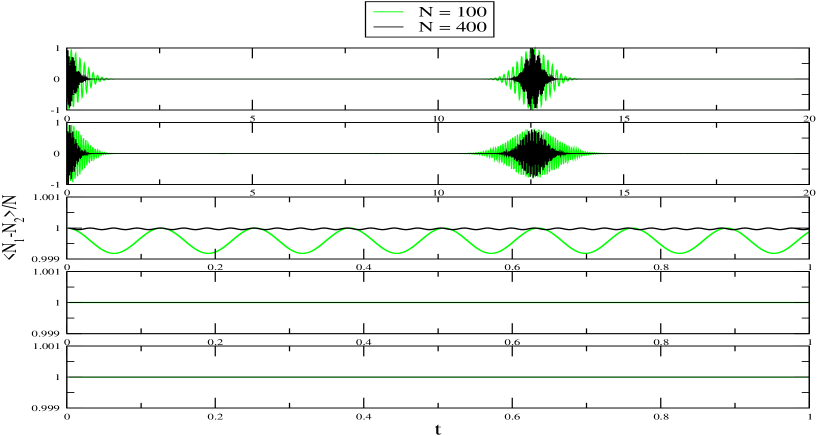
Figure 4: Time evolution of the expectation value for the relative number of particles for different ratios of the coupling $k/{\cal E}_{\mathcal{J}}$ from the top (Rabi regime) to the bottom (Fock regime): $k/{\cal E}_{\mathcal{J}}=1/N^{2},1/N,1,N,N^{2}$ for $N=100,400$ and the initial state is $|N,0\rangle$.

Now we focus in more detail the time evolution of the expectation value of the relative number of particles in the interval $k/{\cal E}_{\mathcal{J}}\in[1/N,1]$ In Fig. 5 we present the case $N=100$: we observe the evolution of the dynamics from a collapse and revival sequence for $k/{\cal E}_{\mathcal{J}}<4/N$, through the self-trapping transition at $k/{\cal E}_{\mathcal{J}}=4/N$, and toward small amplitude harmonic oscillations in the imbalance of the localised state when $k/{\cal E}_{\mathcal{J}}=1$. It is also interesting to observe in the localised phase $k/{\cal E}_{\mathcal{J}}>4/N$ the re-emergence of a collapse and revival sequence. Further increases in $k/{\cal E_{\mathcal{J}}}$ lead to a decaying of the collapse and revival sequence toward harmonic oscillations which occur at $k/{\cal E}_{\mathcal{J}}=1$. A more detailed investigation, using another initial conditions can be found in ref. [13].

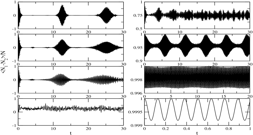
Figure 5: Time evolution of the expectation value between $k/{\cal E}_{\mathcal{J}}=1/N$ and $k/{\cal E}_{\mathcal{J}}=1$. On the left, from the top to the bottom $k/{\cal E}_{\mathcal{J}}=1/N,2/N,3/N,4/N$ and on the right, from the top to the bottom $k/{\cal E}_{\mathcal{J}}=5/N,10/N,50/N,1$, where $N=100$ and the initial state is $|N,0\rangle$.

From the above picture it is clear that the threshold coupling $k/{\cal E}_{\mathcal{J}}=4/N$ predicted by the classical analysis, representing the boundary between a delocalised evolution ($k/{\cal E}_{\mathcal{J}}<4/N$) and self-trapped evolution ($k/{\cal E}_{\mathcal{J}}>4/N$), also holds for the quantum dynamics.

4 Exact Bethe ansatz solution

In this final section we briefly discuss the exact Bethe ansatz solution of (1). More details can be found in [16, 17]. We begin with the $SU(2)$-invariant $R$-matrix, depending on the spectral parameter $u$:

$$R(u)=\left(\begin{array}[]{cccc}1&0&0&0\\ 0&b(u)&c(u)&0\\ 0&c(u)&b(u)&0\\ 0&0&0&1\\ \end{array}\right),$$ (9)

with $b(u)=u/(u+\eta)$ and $c(u)=\eta/(u+\eta)$. Above, $\eta$ is an arbitrary parameter, to be chosen later. It is easy to check that $R(u)$ satisfies the Yang–Baxter equation

$$R_{12}(u-v)R_{13}(u)R_{23}(v)=R_{23}(v)R_{13}(u)R_{12}(u-v).$$ (10)

Here $R_{jk}(u)$ denotes the matrix acting non-trivially on the $j$-th and $k$-th spaces and as the identity on the remaining space.

Next we define the Yang–Baxter algebra $T(u)$,

$$T(u)=\left(\matrix{A(u)&B(u)\cr C(u)&D(u)\cr}\right)$$ (11)

subject to the constraint

$$R_{ab}(u-v)T_{a}(u)T_{b}(v)=T_{b}(v)T_{a}(u)R_{ab}(u-v).$$ (12)

We may choose the following realization for the Yang–Baxter algebra

$$\pi(T_{a}(u))=L_{a1}(u+\omega)L_{a2}(u-\omega),$$ (13)

written in terms of the Lax operators [16]

$$L_{i}(u)=\left(\matrix{u+\eta N_{i}&b_{i}\cr b_{i}^{\dagger}&\eta^{-1}\cr}\right)\;\;\;\;\;\;i=1,2.$$ (14)

Since $L(u)$ satisfies the relation

$$R_{ab}(u-v)L_{ai}(u)L_{bi}(v)=L_{bi}(v)L_{ai}(u)R_{12}(u-v),~{}~{}~{}i=1,\,2$$ (15)

it is easy to check that the Yang-Baxter algebra (12) is also obeyed.

Finally, defining the transfer matrix through

$$t(u)=\pi({\rm tr}_{a}T_{a}(u))=\pi(A(u)+D(u))$$ (16)

it follows from (12) that the transfer matrix commutes for different values of the spectral parameters; i.e., the model is integrable. Now it is straightforward to check that the Hamiltonian (1) is related with the transfer matrix $t$ (16) through

$$H=-\kappa\left(t(u)-\frac{1}{4}(t^{\prime}(0))^{2}-ut^{\prime}(0)-\eta^{-2}+\omega^{2}-u^{2}\right),$$

where the following identification has been made for the coupling constants

$$\frac{k}{4}=\frac{\kappa\eta^{2}}{2},~{}~{}~{}\frac{\Delta\mu}{2}=-\kappa\eta\omega,~{}~{}~{}\frac{\cal{E}_{J}}{2}=\kappa.$$

We can apply the algebraic Bethe ansatz method, using the Fock vacuum as the pseudovacuum, to find the Bethe ansatz equations (BAE)

$$\eta^{2}(v^{2}_{i}-\omega^{2})=\prod^{N}_{j\neq i}\frac{v_{i}-v_{j}-\eta}{v_{i}-v_{j}+\eta}$$ (17)

and the energies of the Hamiltonian (see for example [16, 17])

$$E = -\kappa\left(\eta^{-2}\prod_{i=1}^{N}(1+\frac{\eta}{v_{i}-u})-\frac{\eta^{2}N^{2}}{4}-u\eta N-u^{2}\right.$$ (18)

$$~{}~{}~{}~{}~{}~{}\left.-\eta^{-2}+\omega^{2}+(u^{2}-\omega^{2})\prod_{i=1}^{N}(1-\frac{\eta}{v_{i}-u})\right).$$

Surprisingly this expression is independent of the spectral parameter $u$, which can be chosen arbitrarily.

Using the Bethe ansatz solution, it is possible to derive form factors and correlation functions. Details are given in [16].   

Acknowledgements

AF and GS would like to thank S. R. Dahmen for discussions and CNPq-Conselho Nacional de Desenvolvimento Científico e Tecnológico for financial support. AT thanks FAPERGS-Fundação de Amparo à Pesquisa do Estado do Rio Grande do Sul for financial support. JL gratefully acknowledges funding from the Australian Research Council and The University of Queensland through a Foundation Research Excellence Award.

References

- [1] S. N. Bose, Z. Phys. 26 (1924) 178
- [2] A. Einstein, Phys. Math. K1 22 (1924) 261
- [3] E. A. Cornell and C. E. Wieman, Rev. Mod. Phys. 74 (2002) 875
- [4] J. R. Anglin and W. Ketterle, Nature 416 (2002) 211
- [5] J. Williams, R. Walser, J. Cooper, E. A. Cornell and M. Holland, Phys. Rev. A 61 (2000) 0336123
- [6] M. Albiez, R. Gati, J. Fölling, S. Hunsmann, M. Cristiani and M. K. Oberthaler, Phys. Rev. Lett. 95 (2005) 010402
- [7] A. J. Leggett, Rev. Mod. Phys. 73 (2001) 307
- [8] G. J. Milburn, J. Corney, E. M. Wright and D. F. Walls, Phys. Rev. A 55 (1997) 4318
- [9] S. Raghavan, A. Smerzi, S. Fantoni and S.R. Shenoy, Phys. Rev. A 59 (1999) 620
- [10] S. Kohler and F. Sols, Phys. Rev. Lett. 89 (2002) 060403
- [11] A. P. Tonel, J. Links, and A. Foerster, J. Phys. A: Math. Gen. 38 (2005) 6879
- [12] P. Buonsant, R. Franzosi, V. Penna, J. Phys. B: At. Mol. Opt. Phys. 37 (2004) S229
- [13] A. P. Tonel, J. Links and A. Foerster, J. Phys. A: Math. Gen. 38 (2005) 1235
- [14] A.P. Hines, R.H. McKenzie and G.J. Milburn, Phys. Rev. A 71 (2005) 042303
- [15] F. Pan and J.P. Draayer, Phys. Lett. A 339 (2005) 403
- [16] J. Links, H.-Q. Zhou, R. H. McKenzie and M. D. Gould, J. Phys. A: Math. Gen. 36 (2003) R63
- [17] A. Foerster, J. Links, H.-Q. Zhou, in Classical and quantum nonlinear integrable systems: theory and applications, edited by A. Kundu (Institute of Physics Publishing, Bristol and Philadelphia, 2003) pp 208–233