Failures and avalanches in complex networks

Abstract

We study the size distribution of power blackouts for the Norwegian and North American power grids. We find that for both systems the size distribution follows power laws with exponents $-1.65\pm 0.05$ and $-2.0\pm 0.1$ respectively. We then present a model with global redistribution of the load when a link in the system fails which reproduces the power law from the Norwegian power grid if the simulation are carried out on the Norwegian high-voltage power grid. The model is also applied to regular and irregular networks and give power laws with exponents $-2.0\pm 0.05$ for the regular networks and $-1.5\pm 0.05$ for the irregular networks. A presented mean field theory is in good agreement with these numerical results.

Large transportation networks like the road system, pipelines and the electrical power grid are sensitive to local failures. When failures occur the transport on these networks must be redistributed on the still intact part of the network, occasionally exceeding the local capacity and causing further failures[1, 2]. The resulting avalanches may finally end in major breakdowns: megajams in vehicular traffic or blackouts in the electrical power system.

Such systems get increasingly complex with time as they and the transport on them grow. In addition, the liberalisation of the electrical power distribution market adds more complexity to the power grid system, since the market mechanisms give feedback to the production and transport of power over large regions. As the complexity of these systems increases the ability to predict the behaviour of large unwanted events becomes more and more difficult.

Studies of vulnerability and avalanche statistics in complex networks have been done using different models. In the Motter and Lai model [3] the load on the network is described by betweenness centrality. Avalanches generated by this model on scale free networks were found to follow power law distribution [1]. Alberts et al. studied a similar model on the North American power grid.[4]

Transport properties characterised by conductance for different networks have also been studied on a general basis.[5] And the blackouts in power grids have also been studied in the context of self-organised criticality[2].

The aim of this Letter is to present a model for such systems using the network of the electric power grids and to compare the results with observed data. The electric power distribution system, or power grid, is a system of generators, transformers, power lines and distribution substations. Earlier studies of the North American power grid have found the degree distribution $P(k)\propto e^{-0.5k}$ with mean degree of $2.67$ [4, 6]. We find that the Norwegian power grid also has an exponential degree distribution, but with a mean degree of $2.28$. The number of nodes in he North American power grid is of the order of 15000 nodes (generators, substations,…) whereas the Norwegian one is of the order of 1000 nodes. The difference in mean degree might reflect the fact that Norway is sparsely populated, and have large regions that are only supplied by one or two major grid lines, leading to a smaller value of the mean degree. Power grids are thought to have small world properties, i.e., a large degree of clustering and small characteristic length and where the characteristic path length $l$ scale logarithmically with the number of nodes [6, 7].

The failure distribution has already been studied for the North American power grid [8]. The statistics of the failures will depend on which quantity is used to characterise the size of a failure, either the energy unserved or the power lost. However, both quantities lead to power laws. We will in the following compare the model we present in this Letter to the power loss distribution both for the Norwegian and the North American power grids [10, 9]. We believe that this is the better of the two quantities to use, as the energy unserved will depend on human factors like how long it took to repair a given transmission segment that has broken down.

We present the possibly simplest model which is capable of describing the above mentioned avalanche effects. Imagine a network consisting of electrical conductors, all with the same conductance. One node is picked at random and current will be injected here. Another node, different from the first, will act as a current drain. A potential difference is set up between these two nodes and the Kirchhoff equations are solved to find the current in each link[11]. Once the currents $i$ have been found, we assign a breakdown threshold $t$ to each link such that $t=(1+\alpha)i$, where $\alpha$ is a positive number. The idea here is that each transmission line has been constructed with a fixed tolerance $\alpha$. We found that having more current source/sink pair gave similar results as those found for smaller network, thus effectively reducing the system size.

We now choose a link and remove it in the same way as is done in the random fuse model [12, 13, 14]. The currents are then recalculated. This gives global rearrangement in contrast to the models of self-organised criticality [15] where load rearrangement is local. Some links will at this point carry a current larger than their threshold. These links are then removed from the network and the currents are recalculated once more. Again, the bonds where the current exceeds the threshold are removed and this procedure is repeated until all currents are below the thresholds. This removal process models an avalanche of failures.

Let the conductance between the source and the sink before the initial random removal of a link be denoted by $G_{i}$ and similarly, let $G_{f}$ be the conductance after the avalanche is finished. The difference $\Delta G=G_{i}-G_{f}$ is a measure of the magnitude of the avalanche generated by that removal. If the voltage $V$ between the source and sink nodes is kept fixed during the blackout event, the change in conductance $\Delta G$ will be proportional to the power loss: $\Delta P=P_{i}-P_{f}=V^{2}\Delta G$. For normalisation purposes, we will in the following define $\Delta G=(G_{i}-G_{f})/G_{i}$.

The results we present here are based on generating ensembles of networks and for each network systematically choosing every link as initiator of a blackout event. We study two classes of networks: Random networks with exponential degree distribution, $P(k)\propto e^{-0.5k}$ which is the same as for the Norwegian and North American networks, and small world networks [16] with mean degree $2.67$. Both these network classes have a mean shortest distance $l$ that scale logarithmically with the system size.

We also study square and triangular lattices with bi-periodic boundary conditions, where $l$ grows as the square root of the number of nodes. In addition to these networks and lattices we implement the model on networks with the topology from the Norwegian and North American power grid.

We did simulations for network sizes up to 5041 nodes for the four different artificial network types described above, using the conjugate gradient algorithm to solve the Kirchhoff equations on the network using an error-criterion of $10^{-16}$ [11]. We find that the random and the small world networks give power law probability distributions for the conductance loss $p(\Delta G)\sim\Delta G^{-\gamma}$, as does simulations on the network based on the Norwegian power grid. The regular lattices also give rise to power laws, but with a different value for $\gamma$. It is worth noting that in a study of a somewhat related model by Roux et al. [17], power laws were observed. In that model, a square lattice between two parallel bus bars are gradually depleted by the randomly removing link by link and recording in a histogram the conductance changes between each removal. The scaling of the conductance changes could be traced back to the increasing connectivity length during the process. In this depletion process the thresholds are uncorrelated with the initial currents, while in our case the threshold and initial current distributions are identical.

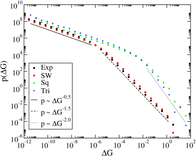
Figure 1: Probability density function of conductance losses for different network and lattice types. The data for the regular lattices have been moved two orders of magnitude towards the right to separate them from the irregular networks. (Exp = exponential network, SW = small world network, Sq = square lattice, Tri = triangular lattice). Some data points for the irregular network have $\Delta G>1$ since the data is put at the midpoints of the logarithmic bins.

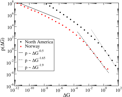
Figure 2: Our model implemented on the Norwegian (1220 nodes) and North American Power (4941 nodes) grids. The straight lines correspond to the power laws observed in the data of fig. 5.

We show in fig. 1 the probability density of conductance changes $\Delta G$ for the random exponential, the small world networks and for the two regular networks. We find that the conductance changes follow power laws in two different regimes. There is a small-event regime characterised by $p(\Delta G)\sim\Delta G^{-0.5}$. The exponent $-0.5$ seems to be independent of network or lattice type. The large-event regime is characterised by two different power laws. The irregular networks follow a power law characterised by an exponent $-1.5\pm 0.05$, whereas the regular lattices follow a power law characterised by an exponent $-2.0\pm 0.07$.

The simulations were performed with $\alpha=3.0$. For smaller values of $\alpha$ a large number of the breakdowns broke the system completely with $\Delta G=1.0$, thus destroying the power law tail for large $\Delta G$s. Larger values of $\alpha$ did not change the tail of the distribution. For the real power blackout data the largest events that were recorded removed $5$% of the totalt capacity of the system. This fact supports the use of an $\alpha$ that does not break the system completely i. e. $\Delta G<1$.

For both the random and the small-world networks, we find that the initial current distribution follows a power law, hence giving a power law distribution of the thresholds.

We now present a mean field estimate of the current distribution in an infinite network. Assume that $n(r)$ is the average number of links at a distance $r$ from an arbitrarily chosen origin. $r$ is the graph theoretical distance, which is of the same order of magnitude as the Euclidean one for a lattice. If a current is injected into the network at the origin, the typical current $i(r)$ in a link at a distance $r$ from the origin will be inversely proportional to the average number of links at that distance, $i(r)\propto 1/n(r)$. Since $n(r)$ is a monotonically increasing function of $r$, $i(r)$ is a monotonically decreasing function of $r$: The smaller the $r$, the larger the average current $i(r)$. The number of links carrying a current higher than a given value $i$, i.e., the cumulative current distribution $P(i)$, is then simply given by

$$P(i)\sim\int_{0}^{r(i)}n(r^{\prime})dr^{\prime},$$ (1)

where we have defined $r(i)$ as the solution with respect to $r$ of the equation $i=1/n(r)$.

For the random exponential networks and the small world networks we have that $n(r)\sim e^{\beta r}$ for small $r$. This is shown numerically in fig. 3. Hence, combining this behaviour with eq. (1), we find

$$P(i)\sim\int_{0}^{-(1/k)\ln(i)}e^{\beta r^{\prime}}dr^{\prime}\sim\frac{1}{i},$$ (2)

for large $i$. This is the behaviour we see in fig. 4.

We note here, as support for the mean field argument we have just presented, that for square and triangular networks, where $n(r)\sim 1/r$, the mean field argument gives $P(i)\sim i^{-2}$, which we also verified numerically.

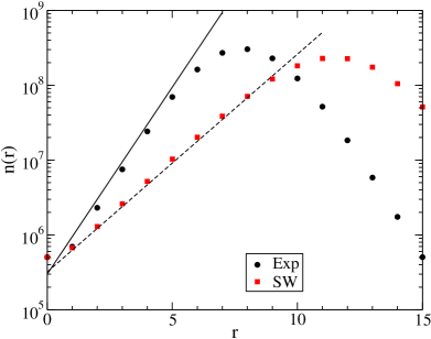
Figure 3: The average number of neighbours $n(r)$ at a distance $r$ for the exponential and the small world networks. $n(r)$ falls of for large $r$ due to the finite size of the networks.

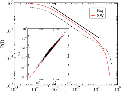
Figure 4: Cumulative current distribution for random exponential and small scale networks each containing 5041 nodes. The distribution function is $P(i)\sim i^{-1}$, as excepted from eq. (2). The inset shows $\Delta G$ vs. $i$. for $\alpha=3.0$. The solid line in the inset is $i^{2}$.

Assume that the resistance $\Delta R$ when a link is broken is much less than the total resistance $R$. With constant voltage difference between the sink and source $\Delta R$ is proportional to $\Delta G$ to the first order of $\Delta G$

$$\Delta R\sim\frac{\Delta G}{G^{2}},$$ (3)

where $G$ is the conductance for the whole system.

Assuming an intermediate length $l$, larger than the lattice constant, but smaller than the system size, Roux et al. [17] argued using Tellegen’s theorem from network theory in electrical engineering [18] that

$$\Delta R=\Delta R_{l}\left(\frac{i_{l}}{I}\right)^{2}$$ (4)

where $\Delta R_{l}$ is the resistance change at scale $l$, $i_{l}$ is the current of a region of scale $l$ and $I$ is the total current. Combining eq. (3) and eq. (4) one gets

$$\Delta G_{j}\sim i_{j}^{2}$$ (5)

which describes the relation between the conductance loss to the system when bond $j$ is removed and $i_{j}$ is the current through the bond. We show the correlation between conductance change $\Delta G_{j}$ and the current $i_{j}$ during the breakdown process for our model in the inset of fig. 4.

With the cumulative current probability shown in fig. 4 and using eqs. (2) and (5) we would expect a distribution function $p(\Delta G)\sim\Delta G^{-1.5}$ for the exponential and small world networks, which is indeed what was observed in fig. 1. We also find that the above argument also predicts the correct distribution function for the regular networks in fig. 1, $p(\Delta G)\sim\Delta G^{-2.0}$.

We note that this argument is based on each breakdown event only involving a single bond. If there is a typical or dominating current carried by the bonds in the avalanches involving more than one bond — and a corresponding conductance change, the argument we have presented carries over to this situation.

The power law for small events, $p(\Delta G)\sim\Delta G^{-0.5}$ in fig. 1 corresponds to a uniform distribution function for the corresponding currents, when using eq. (5).

Finally, we compare the results from our simulations with blackout data from the Norwegian main power grid and data from the largest blackouts in the North American power grid [9, 10]. These data are different due to the fact that the North American data set only look at large events $\Delta P>10$ MW, while the Norwegian data set is for $\Delta P>0.1$ MW.

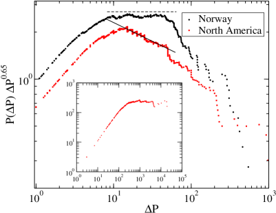
Figure 5: a) Cumulative distribution $P(\Delta P)$ for blackout events $\Delta P$ in the Norwegian (373 events) and North American (390 events) power grids. b) $P(\Delta P)\Delta P^{0.65}$ for blackout events $\Delta P$ in the Norwegian and North American power grids. The straight line to the left following the North American data has an exponent of $-0.24$.

The power blackout data from the main Norwegian central power grid was collected for the period 1995-2005. The North American data span the period 1984-2002. In fig. 5, we show the cumulative probability $P(\Delta P)$ giving the probability to find an event larger than or equal to $\Delta P$. This function is extracted from the data by ordering them in a ascending sequence and then plotting event $k$ in the sequence along the abscissa together with $k/(N+1)$ along the ordinate, where $N$ is the total number of events [19].

In fig. 5, we have shifted the data North American data from fig. 5 to simplify the comparison of the data. The cumulative probability has furthermore been multiplied by $\Delta P^{0.65}$. The ensuing flat plateau in the Norwegian 1995–2005 data suggests that the probability density follows a power law of the form $p(\Delta P)\sim\Delta P^{-1.65}$. For large values of $\Delta P$ it falls off faster. The North American data do not show such a plateau. However, they are consistent with a law regime corresponding to $p(\Delta P)\sim\Delta P^{-1.9}$. The inset shows $P(\Delta P)\Delta P^{1.05}$ which indicates a power law of the form $p(\Delta P)\sim\Delta P^{-2.05}$ for the North American data supporting a exponent $-2$ for this blackout distribution without a cut-off for large $\Delta P$s.

We show in fig. 2 an implementation of our model on the Norwegian and North American power grids[20]. We have fitted power laws to the distribution with exponents $-1.65$ and $-1.9$. These are the power laws that were observed in the blackout histograms shown in fig. 5. We see that the model produces data that are consistent with the observations for the Norwegian power grid, while the data for the North American power grid is inconclusive. It is furthermore interesting to observe that the exponents occurring in the data for moderately sized blackouts lie in between the results of the model implemented on the irregular networks (exponent -1.5) and the regular lattices (exponent -2). The model does not reproduce the large scale blackout distributions for the Norwegian power grid which fall of faster than $\Delta P^{-1.65}$. We also see a small scale regime as for the artificial networks in fig. 1. Hence, the simple model we have introduced is capable to reproduce some aspects of the observed blackout distribution quantitatively with reasonable precision.

The difference for large $\Delta P$s in the Norwegian and the North American datasets could be accounted for by the fact that the North American data also includes large events like snowstorms, hurricanes, while the Norwegian data do not include these events. The difference in nature of widespread events like a hurricane compared with a power line fault can be the cause of the cut off in the Norwegian dataset. This could also be the reason why the exponent for the Norwegian power grid is close to the theoretical value for irregular networks since this argument is based on breaking single links.

The reason why there is a difference in the conductance loss distributions for the simulation with the Norwegian and the North American power grid is not clear. There are however some differences between these two networks when we look at more than just the degree distribution. We observed two differences in $n(r)$ for these to power grids. First $n(r)$ for the Norwegian network is closer to an exponential than the North American network for small $r$ values, and there is a more pronounced peak in $n(r)$ for the Norwegian network, while the North American network have relatively wide plateu. This could explain the difference in $p(\Delta G)$ found in the simulations done on these networks.

We thank Statnett and R. K. Mork for providing us with the Norwegian breakdown data — and NVE and A. E. Grønstvedt for data on the Norwegian power grid. J.Ø.H.B. thanks Ingve Simonsen for discussions on creating probability distributions. This work was partially supported by OTKA K60456 and the Norwegian Research Council. A.H. thanks the Collegium Budapest for hospitality during the period when this work was initiated.

References

- [1] E. J. Lee, K. -I. Goh, B. Kahng and D. Kim, Phys. Rev. E, 71, 056108 (2005)
- [2] M. L. Sachtjen, B. A. Carreras and V. E. Lynch, Phys. Rev. E, 61, 4877 (2000)
- [3] A. E. Motter and Y. -C. Lai, Phys. Rev. E, 66 065102(R) (2002)
- [4] R. Albert, I. Albert and G.L. Nakarado, Phys. Rev. E, 69, 025103(R) (2004).
- [5] López E. Buldyrev S. V. , Havlin S. and Stanley H. E. , Phys. Rev. Lett. 94, 2487011 (2005).
- [6] D.J. Watts and S.H. Strogatz, Nature, 393 440 (1998).
- [7] M.E.J. Newman. SIAM Review, 46, 167, (2003).
- [8] B.A. Carreras, D.E. Newman, I. Dobson and A.B. Poole, in Proceedings of the 33rd Hawaii International Conference on System Sciences – 2000, (IEEE, 2000); B.A. Carreras, D.E. Newman, I. Dobson and A.B. Poole, in Proceedings of the 34rd Hawaii International Conference on System Sciences – 2001. (IEEE, 2001); J. Chen, J.S. Thorp and M. Parashar, in Proceedings of the 34rd Hawaii International Conference on System Sciences – 2001. (IEEE, 2001); B.A. Carreras, D.E. Newman, I. Dobson and A.B. Poole, IEEE Transactions on Circuits and Systems – I: Re. Papers, 51, 1733 (2004).
- [9] Data for the Norwegian blackouts was provided by Statnett.
-
[10]
Data for the North American blackouts can be found at
http://www.nerc.com/ dawg/database.html - [11] G.G. Batrouni and A. Hansen, J. Stat. Phys. 52, 747 (1988).
- [12] L. de Arcangelis, S. Redner and H. J. Herrmann, J. Physique, 46, L585 (1985).
- [13] H. J. Herrmann and S. Roux (Eds.), Statistical Models for the Fracture of Disordered Media (North-Holland, Amsterdam, 1990).
- [14] A. Hansen, Computing in Sci. Eng. 7 (5), 90 (2005).
- [15] P. Bak, How Nature works, Copernicus, New York, 1999
- [16] M. E. J. Newman and D. J. Watts Phys. Lett. A, 263, 341 (1999).
- [17] S. Roux, A. Hansen and E.L. Hinrichsen, Phys. Rev. B, 43, 3601 (1991).
- [18] Tellegen’s Theorem and Electrical Networks, Penfield P. Spencer R. and Duinker S. , MIT Press, Cambridge, 1970.
- [19] Order Statistics, David H. A. ,John Wiley, New York, 1981.
- [20] The Norwegian grid was provided by the Norwegian Water Resource and Energy Directorate NVE, and the the North American grid we used the data at http://cdg.columbia.edu/cdg/datasets.