Partial entropy in finite-temperature phase transitions

Abstract

It is shown that the von Neumann entropy, a measure of quantum entanglement, does have its classical counterpart in thermodynamic systems, which we call partial entropy. Close to the critical temperature the partial entropy shows perfect finite-size scaling behavior even for quite small system sizes. This provides a powerful tool to quantify finite-temperature phase transitions as demonstrated on the classical Ising model on a square lattice and the ferromagnetic Heisenberg model on a cubic lattice.

Recently, it is found that quantum phase transitions can be quantified from the inflexions of the quantum entanglement measures qpt1 ; qpt2 ; qpt3 ; qpt4 ; qpt5 ; qpt6 ; qpt7 ; qpt8 ; qpt9 ; qpt10 . Close to the quantum critical point, the von Neumann entropy, a measure of the quantum entanglement, shows finite-size scaling behavior. This method is quite powerful and straightforward for finding quantum phase transitions in quantum models because one needs neither a pre-assumed order parameter nor a considerable large system size. A natural question arises: Is it possible to generalize this method to quantify finite-temperature phase transitions in thermodynamic systems?

There are several established methods to investigate the finite-temperature phase transitions, such as exact solutions, mean field approach, series expansion, renormalization group analysis, and numerical evaluation of the partition function or correlation functions. However, each known method has its shortcoming. Only few models are exactly soluble. The mean field approach needs a pre-assumed order parameter and may not be reliable. All the numerical methods and the renormalization group analysis need to study large system sizes with complicated computation processes. Therefore, it is highly desirable to find an efficient and general method to characterize finite-temperature phase transitions in both quantum and classical systems.

In this Letter, we point out that the partial entropy, a counterpart of the von Neumann entropy for thermodynamic systems, captures the common feature of all phase transitions, i.e., the information of critical fluctuations. With two models (one classical and one quantum), we show that close to the critical temperature the derivative of the partial entropy shows perfect finite-size scaling behavior even for quite small system sizes. The critical temperature and critical exponents can be determined by the inflexion or the scaling law of the partial entropy. This provides a powerful tool to quantify finite-temperature phase transitions in a variety of interesting models in condensed matter physics.

In the study of quantum phase transitions, one is concerned with the ground state properties as described by the density matrix $|\Psi_{0}\rangle\langle\Psi_{0}|$. Crucial information on quantum correlation or entanglement between a subsystem $p$ and the rest $\bar{p}$ exists in the reduced density matrix $\rho_{p}(\alpha)\equiv tr_{\bar{p}}|\Psi_{0}\rangle\langle\Psi_{0}|$, as is captured in the von Neumann entropy, $E_{v}=-tr\rho_{p}\ln\rho_{p}$. It has been shown that singular behavior in the von Neuman entropy occurs as a function of control parameters as the system goes through a quantum phase transition qpt0 .

The concept of von Neumann entropy can be straightforwardly generalized to thermodynamic systems at finite temperatures $T$. The density matrix now reads $\rho(T)=\exp{(-H/T)}/Z$, where $H$ is the Hamiltonian, and $Z$ is the partition function. One can similarly define a reduced thermal density matrix $\rho_{p}(T)=tr_{\bar{p}}\rho(T)$, and consider the partial entropy $S_{p}(T)\equiv-tr\rho_{p}(T)\ln\rho_{p}(T)=-\sum_{n=1}^{D_{H}}p_{n}\ln p_{n}$, where $D_{H}$ is the dimension of the Hilbert space of the subsystem $p$, and $p_{n}$ are the eigenvalues of $\rho_{p}(T)$. For a classical system, the trace operation is replaced by summing over the classical states. The partial entropy is determined by the probability distribution of the subsystem. It also measures the quantum and classical correlation between the subsystem and the rest of the system. As is shown below, the partial entropy in fact captures the main feature of the critical fluctuation and therefore shows singular behavior close to the critical temperature. Its inflexion gives the information of the critical point.

As our first example, we study the two-dimensional (2D) Ising model. It is well known that this system is exactly soluble, undergoing a second order phase transition tc at $T_{c}=2/$arcsinh$(1)\approx 2.26919J/k_{B}$ and its critical behaviors have been studied very well. It is therefore an ideal system to test our method. The Hamiltonian is $H=-\sum_{\langle ij\rangle}\sigma_{i}^{z}\sigma_{j}^{z}$, where $\sigma_{i}^{z}=\pm 1$ is the spin along $z$-direction on site $i$ and $\langle ij\rangle$ indicates bonds between nearest neighbor sites.

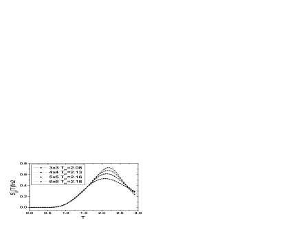
Figure 1: The derivative of the partial entropy $S^{\prime}_{p}(T)$ versus temperature for $L=3-6$ are plotted. A maximum appears at certain temperature $T_{m}$ for a given $L$. On increasing $L$, the peak becomes more pronounced and $T_{m}$ shifts accordingly to the critical temperature of the 2D Ising model $T_{c}=2.26919$.

We consider the $L\times L$ square-lattice case and use the periodic boundary condition. We focus our attention on the subsystem of two nearest neighbor sites. The reduced density matrix is obtained by tracing all the spins except those two. Since the system is translational invariant, $\rho_{p}(T)$ is independent of the choice of the bond and takes the form $\rho_{p}(T)=[1+\gamma(T)\sigma_{1}^{z}\sigma_{2}^{z}]/4$ by a simple symmetry analysis, where $\gamma(T)$ is a parameter depending on the temperature and system size $L$. Then we obtain the partial entropy as

$$S_{p}(T)=2\ln 2-\frac{1}{2}\left\{\gamma\ln\frac{1+\gamma}{1-\gamma}+\ln[1-\gamma^{2}]\right\}.$$ (1)

Thermal fluctuations increase with temperature, so does the partial entropy. When $T\to 0$, the spins are ordered either up or down. The parameter $\gamma(0)=1$ and the partial entropy takes the minimum value of $\ln 2$. At extremely high temperatures $T\to\infty$, all the four states have the same probability to occur. In this case $\gamma(\infty)=0$ and the partial entropy takes the maximum value $2\ln 2$. The partial entropy increases monotonically between these two extreme values which are independent of L. More interestingly, the derivative of the partial entropy $S^{\prime}_{p}(T)$ has a maximum, corresponding to fastest growth of the partial entropy. The peak at the maximum sharpens as the system size increases (Fig. 1), and the maximum value diverges logarithmically with the system size (Fig.2). This singular behavior indicates a critical point of our system.

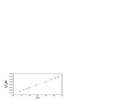
Figure 2: The maximum values of the derivative of the partial entropy $S^{\prime}_{p}(T_{m})$ for $L=3-6$ (black dots) depend linearly on $\ln L$ (dotted line). Monte Carlo results for larger $L=10,20,30,40,50$ (circles) fall on this straight line, confirming the logarithmic divergence for a second-order phase transition.

Figure 3: The peak temperature $T_{m}$ versus logarithm of the system size is depicted to quantify the phase transition temperature $T_{c}$. The black dots for $L=3-6$ are from the exact numerical calculation while the circles for larger $L=10,20,30,40,50$ are from the Monte Carlo simulation. The dotted line is a fit with the formula $T_{m}=2.27802-0.58995L^{-1}$ from the $L=3-6$ data only. The $L\to\infty$ limit is very close to the exact value 2.26919.

Exact calculations are performed for system sizes $L=3-6$, and Monte Carlo simulations are done for large sizes up to $L=50$. The straight line fit in Fig.2, $S^{\prime}_{p}(T_{m})=0.42034\ln L+{\text{c}onst,}$ is from the first four points, and it is also followed nicely by the Monte Carlo data. The temperature $T_{m}$ at the peak of $S^{\prime}_{p}(T)$ shows a size dependence linear in $1/L$ (Fig.3). Just from the first four points, we find the fit $T_{m}=2.27802-0.58995L^{-1}$, which turns out to be also well followed by the Monte Carlo data for larger sizes. A critical temperature, $T_{c}=2.27802$, is extracted from the above fit as the limiting value of $T_{m}$ at $L\to\infty$. This is very close to the exact value of $2.26919$. We have thus seen the effectiveness of the partial entropy method in providing accurate information on the critical point from fairly small system sizes.

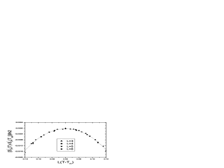
Figure 4: The finite size scaling of the partial entropy is performed. The deviation of the first derivative of the partial entropy from its maximum is only a function of $L(T-T_{m})$. All the data from $L=3$ to $L=6$ fall on a single curve, indicating a perfect scaling behavior of the partial entropy around the critical temperature.

We can also study the scaling behavior of the partial entropy as a function of both the system size and temperature. We observe that $S^{\prime}_{p}(T)-S^{\prime}_{p}(T_{m})\sim Q[L(T-T_{m})]$, where the scaling function $Q(x)\sim C_{\infty}\ln x$ for large $x$, and $Q(x)\sim 0$ for very small $x$ scale . We find that all the data from different system sizes $L$ converge to a single curve, which is shown in Fig.4. These results establishes that finite size scaling is present in the partial entropy.

There is a direct relationship between the partial entropy and thermodynamic quantities, which explains why singular behavior of the partial entropy can be used to characterize the critical point and associated scaling properties. We observe that the density of internal energy may be found as $u(T)=L^{-2}trH\rho(T)=-2tr_{p}\rho_{p}(T)(\sigma_{1}^{z}\sigma_{2}^{z})=-2\gamma(T)$. Therefore, the partial entropy Eq.(1) can be determined uniquely by the internal energy density $u$. Moreover, the derivative of the partial entropy can be found as $S^{\prime}_{p}(T)=Tds(T)\ln[(2-u)/(2+u)]/(4dT)$, where $s(T)$ is the density of entropy of the whole system and we have used the thermodynamic relation $du/dT=Tds/dT$. In the neighborhood of the critical point, the internal energy density $u$ lies somewhere in the middle of the interval $(-2,0)$ and varies smoothly with temperature (with continuous first derivative). Therefore, the singular point of $S^{\prime}_{p}(T)$ coincides with that of the derivative of the global entropy density $s(T)$. Therefore, one can indeed use the partial entropy to quantify thermodynamic phase transitions.

Moreover, the partial entropy is a quantity more suitable for finite-size studies than standard thermodynamic quantities, in that scaling behavior sets in much earlier in the former than in the latter. This allows precise determination of the critical temperature, for example, from relatively small system sizes using our method. For contrast, we performed finite-size calculations for $ds/dT$, finding that its maximum in the temperature dependence diverges as a polynomial rather than a linear function of $\ln L$. Also, the peak temperature $T_{m}$ of $ds/dT$ is nonlinear in $1/L$. The data for $L=3-6$ can be nicely fitted (with an error less than 0.001) by the function $T_{m}=2.3373-1.50437L^{-2.493}$. However, its extrapolation (2.3373) to infinite size is far from the true critical temperature. One may take this to mean that the coefficients and the exponent of such a fit are modulated slowly in $L$ (such as logarithmic). Another interpretation is that there are subdominant terms in finite-size scaling which do not decay quickly with the system size. In any case, it is very clear that one cannot obtain useful results from thermodynamic quantities when the system sizes are not very large. On the other hand, the partial entropy does seem to be free from such complications.

It remains to be explained why the partial entropy is superior to the global entropy in finite-size scaling. At this moment, we do not have a clear answer, but offer the following observation which may shed some light to this question. The basic ingredient of the partial entropy method is quite similar to that of the renormalization group transformation. As is well known, in the later approach, information about the critical fluctuation remains unchanged, because the critical point is a fixed point of the renormalization group transformation. The partial entropy captures the essence of critical fluctuations of the system.

So far we have been concerned with a classical system, we consider next a quantum Heisenberg model on a cubic lattice. In this model, the critical fluctuation is much weaker than that in the 2D Ising model, because the critical divergence follows a power law in the former while it follows a logarithmic law in the latter. However, the partial entropy method still works very well in this quantum system. The Heisenberg Hamiltonian reads, $H=-2\sum_{\langle ij\rangle}{\vec{S}}_{i}\cdot{\vec{S}}_{j}$, where ${\vec{S}}_{i}={\vec{\sigma}}_{i}/2$ is the spin-1/2 operator and $\langle ij\rangle$ indicates bonds between nearest neighbor sites. This model has a second-order phase transition at the critical temperature $T_{c}=1.6778\pm 0.0002$ as determined by high-accuracy quantum Mote Carlo simulation and phenomenological renormalization-group analysis souza .

The reduced density matrix for a nearest neighbor pair of sites can again be found in a simple form, $\rho_{p}(T)=1/4-[2u(T)/9]{\vec{S}}_{1}\cdot{\vec{S}}_{2}$, based on a symmetry analysis corr ; hai . Its coefficient is related to the internal energy density $u(T)$ by tracing the reduced density matrix with the Hamiltonian. The partial entropy can then be expressed as $S_{p}(T)=-\{[9-2u][\ln(9-2u)-2\ln 6]+[3+2][\ln(3+2)-\ln 12]\}/12$. These expressions remain valid for finite system sizes under periodic boundary conditions. We use quantum Mote Carlo simulation with a stochastic series expansion algorithm mon to calculate the density of internal energy and then to obtain the partial entropy from the above formula.

We will show that this critical temperature can be obtained accurately by using the partial entropy method with the calculation for small-size system.

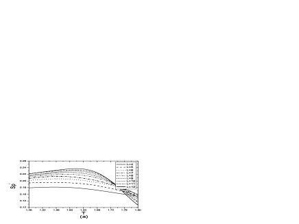
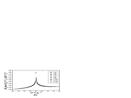
Figure 5: (a) The derivative of partial entropy shows a peak at certain temperature. (b) The finite-size scaling of the derivative of partial entropy.

As before, the partial entropy is monotonically increasing with $T$, while its derivative $S^{\prime}_{p}(T)$ arrives at a maximum at certain temperature. The peaks of $S^{\prime}_{p}(T)$ for linear sizes of $L=4-12$ are shown in detail in Fig. 5(a). The peaks sharpen with increasing $L$, and suppose to become singular at $L\rightarrow\infty$. The different curves can be collapsed on to a single one, shown in Fig. 5(b), by the following scaling relation

$$S^{\prime}_{p}(\infty)=S^{\prime}_{p}(L)+gL^{\alpha/\nu},$$

$$[S^{\prime}_{p}(t,L)-S^{\prime}_{p}(\infty)]|t|^{\alpha}=f(tL^{1/\nu}),$$ (2)

where $t=1-T/T_{c}$, $f$ is an universal function and $g$ is a constant. Our result yields the critical exponents $\alpha=-0.1116\pm 0.0005$, $\nu=0.705\pm 0.003$ and the critical temperature $T_{c}=1.677\pm 0.001$, which agree very well with those obtained earlier le ; souza .

More remarkably, the finite-size scaling for the partial entropy starts to work from relatively small system sizes. If we use data only from $L=4-8$, the fitting to a scaling function then yields $\alpha=-0.703\pm 0.003$, $\nu=0.1196\pm 0.0005$ and $Tc=1.678\pm 0.002$, which are already very good. On the other hand, thermodynamic quantities, such as the specific heat, show good scaling behavior only for $L\geq 8$ sandv .

In conclusion, we suggest that the partial entropy is quite an effective tool to quantify the finite-temperature phase transitions. The critical temperature can be determined by the inflexion of the partial entropy or the peak of its derivative with respect to temperature. The partial entropy shows good finite-size scaling even for relatively small system sizes. The key point lies in the fact that the partial entropy catches the most essential feature of phase transitions, i.e., the information of critical fluctuations. The advantages of this method are: one does not need a pre-assumed order parameter; does not need to study a special large-scale correlation function, and it is straightforward and efficient. Elements of the partial entropy are closely related to the thermodynamic quantities or correlation functions via simple symmetry analysis.

J. Cao and Y. Wang are supported by NSFC under grant No.10474125, No.10574150 and the national key project on basic research. Q. Niu is supported by the NSF and the R.A. Welch Foundation.

^∗Electronic address: yupeng@aphy.iphy.ac.cn

References

- (1) A. Osterloh et al., Nature 416, 608 (2002).
- (2) T.J. Osborne et al., Phys. Rev. A 66, 032110 (2002).
- (3) S.J. Gu et al., Phys. Rev. A 68, 042330 (2003).
- (4) G. Vidal et al., Phys. Rev. Lett. 90, 227902 (2003).
- (5) H. Barnum et al., Phys. Rev. A 68, 032308 (2003).
- (6) F. Verstraete et al., Phys. Rev. Lett. 92, 027901(2004).
- (7) R. Somma et al., Phys. Rev. A 70, 042311 (2004).
- (8) T. Roscilde et al., Phys. Rev. Lett. 93, 167203 (2004).
- (9) M. Popp et al., Phys. Rev. A 71, 042306 (2005).
- (10) T. Roscilde et al., Phys. Rev. Lett. 94, 147208 (2005).
- (11) See, for example, S.Q Su et al., Phys. Rev. A 74, 032308 (2006), and the references therein.
- (12) L. Onsager, Phys. Rev. 65, 117 (1944); B. Kaufman, Phys. Rev. 76, 1232 (1949); T.D. Schultz et al., Rev. Mod. Phys. 36, 856 (1964).
- (13) L.-A. Wu et al., Phys. Rev. Lett. 93, 250404 (2004).
- (14) M.F. Yang, Phys. Rev. A 71, 030302(R) (2005).
- (15) M.N. Barber, in Phase Transitions and Critical Phenomena Vol. 8, edited by C. Domb and J.L. Leibovitz (Academic Press, London, 1983).
- (16) A.J.F. de Souza et al., Phys. Rev. B 62, 8909 (2000); I.V. Rojdestvenski et al., Phys. Rev. B 56, 2698 (1997).
- (17) See, for example, T. Tanaka, Methods of statistical physics (Cambridge University Press, Cambridge, 2002).
- (18) S.J. Gu et al., Phys. Rev. Lett. 93, 086402 (2004).
- (19) A.W. Sandvik, Phys. Rev. B 56, 11678 (1997); Phys. Rev. B 59, R14157 (1999).
- (20) J.C.Le Guillou et al., Phys. Rev. B 21, 3976 (1980).
- (21) A.W. Sandvik, Phys. Rev. Lett. 80, 5196 (1998).