Critical Velocities for Energy Dissipation from Periodic Motions of Impurity in Bose-Einstein Condensates

Abstract

A phenomenon of energy dissipation in Bose-Einstein condensates is studied based on a microscopic model for the motion of impurity. Critical velocities for onset of energy dissipation are obtained for periodic motions, such as a dipole-like oscillation and a circular motion. The first example is similar to a series of MIT group experiments settings where the critical velocity was observed much below the Landau critical velocity. The appearance of the smaller values for the critical velocity is also found in our model, even in the homogeneous condensate in the thermodynamic limit. This suggests that the landau criterion be reexamined in the absence of quantized vortices in the bulk limit.

I Introduction

In 1941 Landau gave a phenomenological argument about the critical velocity in a superfluid below which no energy dissipations occur landau . His argument was entirely based on a kinematics and the Galilean invariance. This critical velocity is now known as the Landau criterion, which states that if impurities in a superfluid move slower than $v_{c}=\min\omega({\bm{p}})/|{\bm{p}}|$, then there are no excitations created in a superfluid. Here $\omega({\bm{p}})$ is the dispersion relation of excitations with the momentum ${\bm{p}}$. This then explains the phenomenon of the superfluidity. In a real superfluid, however, finite energy dissipations take place even below the Landau critical velocity. This is due to creation of quantized vortices, which was explained later by Feynman feynman . A microscopic understanding of the superfluidity was initiated by Bogoliubov bogoliubov47 . He particularly showed that the phenomenon of superfluidity can be explained as a consequence of condensation of massive bosons in the ground state. Although his model cannot be strictly speaking, applied to the real ⁴He due to strong interactions between atoms, he succeed to explain the Landau criterion from the first principle. Bogoliubov’s weakly interacting massive boson model has been studied extensively in more than half century bru .

The celebrated experimental realization of Bose-Einstein condensates (BECs) in several alkali vapors have revived theoretical works on BECs as well as experimental works bec ; review . Particularly, the mean field approximation of the Bogoliubov model, the Gross-Pitaevskii equation, has been studied extensively review . One reason is because this model can be adopted as a realistic model. Another reason is that the current experimental technics are remarkably well developed and under controlled to provide variety of opportunities to test these theories. Indeed, so far theories have good agreements with experimental results in many cases. However, there are still experimental facts which are left without satisfactory explanation. In this paper we would like to give analytical argument to one of those experiments. They are a series of experiments done by MIT group mit1 ; mit2 ; mit3 .

These experiment were intended to examine the Landau criterion in BECs. Interestingly, they have found disagreement with Landau’s argument. The essence of these experiments is as follow. The sodium condensate was created in anisotropic harmonic traps forming an elongated in one axial direction. A Gaussian laser beam was then used to stir the condensate by moving it back and forth periodically. The critical velocity for creating energy dissipation was observed less ten times smaller than the Landau critical velocity. Since a publication of these experimental results, there appear many theoretical works to fulfill this discrepancy. One of the important question is whether this experimental fact is due to the bulk property of BECs or is originated from other factors, such as creation of vortices jackson , the geometry of the condensate fedichev , and so on ref . There is no doubt about the fact that all these factors give rise to the experimental observations of energy dissipations below the Landau critical velocity. However, there still remain unclear whether this discrepancy may happen in the homogeneous system.

In this paper we argue that the appearance of the smaller critical velocity is also part of the bulk properties of the condensates. Hence this effect does occur even in the homogeneous system in the thermodynamic limit as contrast to the original Landau’s argument. To demonstrate it we will evaluate the critical velocity for the energy dissipation in the homogeneous BEC in the thermodynamics limit at zero temperature. To capture the physics of MIT experiments, we couple the weakly interacting bosons with an external impurity whose trajectory is given by a periodic motion similar to the actual experiment. We show that this model provides qualitative understandings of the discrepancy observed in laboratories. We also compare the result with other possible periodic motion, a circular motion. The result shows that the same conclusion holds for the case of the circular motion. A comparison between two cases suggests that the circular motion has more dissipation than the dipole-like oscillation and the larger critical velocity.

The paper continues as follows. In Sec. II we give a summary of our model and its solution within the Bogoliubov approximation. A formula for the energy dissipation due to the motion of impurity in BECs is also given. An idealized case of MIT group experimental settings is studied and the critical velocity is evaluated in Sec. III. In Sec. IV energy dissipation from a circular motion and its comparison to the result of Sec. III are given. Sec. V gives a summary and discussion of our results.

II The Model and Its Solution

II.1 The model Hamiltonian and its diagonalization

The model for motions of classical impurities in the homogeneous BEC was proposed and studied in ms ; jun1 ; jun2 . We give a summary of result together with the essence of the model. The total Hamiltonian is the sum of two parts. One is the standard Bogoliubov weakly interacting massive bosons term $\hat{H}_{B}$, and the other is the interaction term $\hat{H}_{I}$ between bosons and a moving impurity which takes into account the local interaction between them :

$$\hat{H}_{B}=\int\!d^{3}x\;\hat{\psi}^{\dagger}({\bm{x}},t)(-\frac{\hbar^{2}{\bm{\nabla}}^{2}}{2M})\hat{\psi}({\bm{x}},t)\\ +\frac{g}{2}\int\!d^{3}x\;\hat{\psi}^{\dagger}({\bm{x}},t)\hat{\psi}^{\dagger}({\bm{x}},t)\hat{\psi}({\bm{x}},t)\hat{\psi}({\bm{x}},t),$$ (1)

where $M$ is the mass of the bosons. The coupling constant $g$ between bosons is expressed in terms of the s-wave scattering length $a_{s}$; $g=4\pi a_{s}\hbar^{2}/M$. We assume the repulsive interaction $g>0$ and diluteness $na_{s}^{3}\ll 1$ with $n$ the number density of bosons. The interaction term is

$$\hat{H}_{I}=\lambda\int d^{3}x\;\rho_{c}({\bm{x}},t)\hat{\psi}^{\dagger}({\bm{x}},t)\hat{\psi}({\bm{x}},t).$$ (2)

Here $\lambda$ is the coupling constant between bosons and the impurity, and $\rho_{c}({\bm{x}},t)$ is the time dependent distribution of classical impurity. Particularly, we have in mind an idealized point-like disturbance on the condensate guided along a given trajectory ${\bm{\zeta}}(t)$, i.e. we will adopt the replacement $\rho_{c}({\bm{x}},t)=\delta({\bm{x}}-{\bm{\zeta}}(t))$.

In order to estimate the effects of the impurity in the thermodynamics limit, we expand the field operators $\hat{\psi}({\bm{x}},t)$ in terms of the plane wave basis with periodic boundary conditions in a finite size box $V=L^{3}$. The limit $N$ and $V$ go to infinity whit a fixed density $n=N/V$ will be taken at the end of calculations. We follow Bogoliubov’s treatment to simplify the total Hamiltonian $\hat{H}=\hat{H}_{B}+\hat{H}_{I}$ within a number conserving framework of Bogoliubov model comment . After several steps jun2 , we arrived at an approximated Hamiltonian :

$$\hat{H}_{B}=E_{0}+\sideset{}{{}^{\prime}}{\sum}(\epsilon_{k}+gn)\hat{\alpha}_{{\bm{k}}}^{\dagger}\hat{\alpha}_{{\bm{k}}}+\frac{gn}{2}\sideset{}{{}^{\prime}}{\sum}(\hat{\alpha}_{{\bm{k}}}^{\dagger}\hat{\alpha}^{\dagger}_{-{\bm{k}}}+{\rm h.c.})\\ +\frac{n\lambda}{\sqrt{N}}\sideset{}{{}^{\prime}}{\sum}(\tilde{\rho}_{{\bm{k}}}(t)\hat{\alpha}_{{\bm{k}}}^{\dagger}+{\rm h.c.}).$$ (3)

Here $E_{0}=gnN/2-gn/2+\lambda n$ is a constant term, $\epsilon_{k}=\hbar^{2}{\bm{k}}^{2}/2M$ is the free kinetic energy of bosons, and $\tilde{\rho}_{{\bm{k}}}(t)=\int d^{3}x\;\rho_{c}({\bm{x}},t)e^{-i{\bm{k}}\cdot{\bm{x}}}$. In this approximation we neglected terms of order of $N^{-1}$.

Bogoliubov’s excitation is created and annihilated by the operators

$$\hat{b}_{{\bm{k}}}^{\dagger} =\hat{\alpha}_{{\bm{k}}}^{\dagger}\cosh\theta_{k}+\hat{\alpha}_{-{\bm{k}}}\sinh\theta_{k},$$ (4)

$$\hat{b}_{{\bm{k}}} =\hat{\alpha}_{{\bm{k}}}\cosh\theta_{k}+\hat{\alpha}_{-{\bm{k}}}^{\dagger}\sinh\theta_{k},$$ (5)

with

$$\theta_{k}=\tanh^{-1}(\frac{gn}{\hbar\omega_{k}+\epsilon_{k}+gn}),\ \hbar\omega_{k}=\sqrt{\epsilon_{k}(\epsilon_{k}+2gn)}.$$ (6)

In terms of Bogoliubov’s excitation, the total Hamiltonian is expressed as

$$\hat{H}=E^{\prime}_{0}+\sideset{}{{}^{\prime}}{\sum}\hbar\omega_{k}\hat{b}_{{\bm{k}}}^{\dagger}\hat{b}_{{\bm{k}}}+\sideset{}{{}^{\prime}}{\sum}{\bm{(}}f_{{\bm{k}}}(t)\hat{b}_{{\bm{k}}}^{\dagger}+{\rm h.c.}{\bm{)}}.$$ (7)

Here $E^{\prime}_{0}=E_{0}+\sideset{}{{}^{\prime}}{\sum}(\hbar\omega_{k}-\epsilon_{k}-gn)/2$ is the ground state energy without impurities (a prime indicates the omission of the zero mode from the summation), and $f_{{\bm{k}}}(t)=n\lambda\tilde{\rho}_{{\bm{k}}}(t)\sqrt{\epsilon_{k}/(N\hbar\omega_{k})}$. Therefore, the fist order impurity effects are equivalent to decoupled forced harmonic oscillators, which can be solved analytically. Since we are solving the time dependent problem, it is natural to work in the Heisenberg picture. The equations of motions for Bogoliubov’s excitation creation and annihilation operators are easily solved as follows.

$$\hat{b}^{\dagger}_{{\bm{k}}}(t) =\hat{B}^{\dagger}_{{\bm{k}}}(t)+\phi^{*}_{{\bm{k}}}(t),$$ (8)

$$\hat{b}_{{\bm{k}}}(t) =\hat{B}_{{\bm{k}}}(t)+\phi_{{\bm{k}}}(t).$$ (9)

Here $\phi_{{\bm{k}}}(t)$ is a $c$-number function :

$$\phi_{{\bm{k}}}(t)=\frac{n\lambda}{i\hbar}\sqrt{\frac{\epsilon_{k}}{N\hbar\omega_{k}}}I_{{\bm{k}}}(t)e^{-i\omega_{k}t},$$ (10)

where the integral $I_{{\bm{k}}}(t)$ is defined by

$$I_{{\bm{k}}}(t)=\int^{t}_{t_{0}}dt^{\prime}\;\tilde{\rho}_{{\bm{k}}}(t^{\prime})e^{i\omega_{k}t^{\prime}}.$$ (11)

We have chosen the boundary condition such that the system is disturbed by impurity at $t=t_{0}$.

Now the our system is described by in terms of the dressed Bogoliubov excitation creation and annihilation operators $\hat{B}^{\dagger}_{{\bm{k}}}$ and $\hat{B}_{{\bm{k}}}$. They evolve according to the diagonalized Hamiltonian $\hat{H}^{\prime}$ :

$$\hat{H}^{\prime}=\tilde{E}_{0}(t)+\sideset{}{{}^{\prime}}{\sum}\hbar\omega_{k}\hat{B}^{\dagger}_{{\bm{k}}}\hat{B}_{{\bm{k}}}.$$ (12)

In the diagonalized Hamiltonian, the new ground state energy is defined by $\tilde{E}_{0}(t)=E^{\prime}_{0}+\sideset{}{{}^{\prime}}{\sum}{\rm Re}{\bm{(}}f_{{\bm{k}}}^{*}(t)\phi_{{\bm{k}}}(t){\bm{)}}$. The energy spectrum $\hbar\omega_{k}$ is that of the gapless excitations characterized by $\omega_{k}\simeq kc_{s}$ for a small $k$, where $c_{s}=\sqrt{gn/M}$ is the speed of sound. We remark that the spectrum $\omega_{k}$ and the speed of sound $c$ are the same as in the original Bogoliubov model without impurities. Hence, the motion of impurities does not affect either $\omega_{k}$ nor $c$ in our model within the above approximation.

II.2 Homogeneous condensate

The homogeneous BEC is defined by the ground state of the Hamiltonian (7) without the impurity term. In other word the vacuum state of the annihilation operators $\hat{b}_{{\bm{k}}}$. We denote it as $|bec\rangle$, and this is to be defined by

$$\hat{b}_{{\bm{k}}}|bec\rangle=0\quad\forall{\bm{k}}\neq 0.$$ (13)

Therefore, we conclude that the dressed Bogoliubov excitation annihilation operator due to impurity does not see the condensate as vacuum :

$$\hat{B}_{{\bm{k}}}|bec\rangle=-\phi_{{\bm{k}}}(t)|bec\rangle.$$ (14)

Alternatively, one can interpret this result as follows. A classical field describe by $\phi_{{\bm{k}}}(t)$ is induced in the homogeneous condensate due to the motion of impurity.

II.3 Energy dissipation due to the motion of impurity

As we have mentioned in Introduction, we are interested in the amount of dissipated energy in condensates due to the motion of impurity. Physically, energy dissipations take place via scattering processes between bosons and impurity. In other words the impurity motion creates excitations in condensates by scattering processes. Excitations in BECs will carry amount of energy equal to their excitation spectra. The amount of dissipated energy is then measured by heat transferred to condensates.

We first define the occupation number for the dressed Bogoliubov’s excitation with respect to the homogeneous condensate. This number counts the emitted Bogoliubov’s excitations accompanying with the motion of impurity in BEC,

$$\tilde{n}_{{\bm{k}}}(t)\equiv\langle bec|\hat{B}^{\dagger}_{{\bm{k}}}(t)\hat{B}_{{\bm{k}}}(t)|bec\rangle=|\phi_{{\bm{k}}}(t)|^{2}$$ (15)

Multiplying by the excitation energy $\hbar\omega_{k}$ gives the dissipated energy ${\cal E}_{{\bm{k}}}(t)$ for a given mode ${\bm{k}}$, and the total dissipated energy ${\cal E}(t)$ is given by summing over all modes. In our model we assume that an impurity is driven by some external forces, in which back reaction is negligible. Therefore, this dissipated energy is equivalent to the amount of energy transfered to the condensate from the external impurity. In the thermodynamic limit, the total energy dissipation due to impurity is evaluated by rather simple formula :

$${\cal E}(t)=\sideset{}{{}^{\prime}}{\sum}{\cal E}_{{\bm{k}}}(t)\to\frac{n\lambda^{2}}{\hbar^{2}}\int\!\frac{d^{3}k}{(2\pi)^{3}}\;\epsilon_{k}|I_{{\bm{k}}}(t)|^{2}.$$ (16)

II.4 Depletion of the condensate

The depletion of the condensate $d(t)$ due to the quantum fluctuation is defined by the formula :

$$d(t)=\sideset{}{{}^{\prime}}{\sum}\langle bec|\hat{\alpha}_{{\bm{k}}}^{\dagger}\hat{\alpha}_{{\bm{k}}}|bec\rangle/N.$$ (17)

Using the Bogoliubov transformation and the solution obtained before,

$$d(t)=\sideset{}{{}^{\prime}}{\sum}\frac{1}{2N}(\frac{\epsilon_{k}+gn}{\hbar\omega_{k}}-1)\\ +\frac{1}{N}\sideset{}{{}^{\prime}}{\sum}(\frac{\epsilon_{k}}{\hbar\omega_{k}}|\phi_{{\bm{k}}}(t)|^{2}+\frac{gn}{2\hbar\omega_{k}}|\phi^{*}_{{\bm{k}}}(t)-\phi_{-{\bm{k}}}(t)|^{2}).$$ (18)

Since $|\phi_{{\bm{k}}}(t)|^{2}$ has an additional factor $1/N$ (see eq. (10)), the motion of impurity does not contribute to the depletion of the homogeneous condensate in the thermodynamic limit. The depletion is then given by $d=(8/3)\sqrt{na_{s}^{3}/\pi}$ which is independent of the impurity effects. Therefore, in the large $N$ limit, the homogeneous condensate is stable against an external impurity. In contrast, however, these terms in the depletion of condensates is not negligible in real experiments where the finiteness of the number of particles and finite size effects play important roles.

III MIT Group Experiments

We now apply our model to the experimental settings done by MIT group. We consider a point-like impurity which is oscillating along the $z$-axis with a period $2\pi/\Omega$ and the oscillation amplitude $d$. The trajectory is expressed by ${\bm{\zeta}}(t)=(0,0,d\cos\Omega t)$. Although this is still an idealized model, we will see that this model gives qualitative explanation for the real experiments. To make the corresponding to the experiments, we also define the velocity of the impurity by $v=2d/\pi\Omega$. In order to obtain analytical expressions for the energy transferred to the condensate, we further make an assumption that the impurity is oscillating for a sufficiently very long time. This assumption seems reasonable if we look the real experimental values. Under this assumption we let the time integral (11) from $-\infty$ to $+\infty$. Using the plane wave expansion in terms of the Bessel function ${\rm J}_{\ell}(x)$, $\exp(-ix\cos\phi)=\sum_{\ell=-\infty}^{\infty}(-i)^{\ell}\exp(i\ell\phi){\rm J}_{\ell}(x)$, we obtain

$$I_{{\bm{k}}}(\infty) =\sum_{\ell=-\infty}^{\infty}(-i)^{\ell}{\rm J}_{\ell}(kd\cos\theta)\int_{-\infty}^{\infty}\!dt\;e^{i\omega_{k}t+i\ell\Omega t}$$ (19)

$$=2\pi\sum_{\ell=1}^{\infty}(-i)^{\ell}{\rm J}_{\ell}(kd\cos\theta)\;\delta(\omega_{k}-\ell\Omega).$$ (20)

Here the wave number vector ${\bm{k}}$ is written in the spherical coordinates with $\theta$ an angle from the $z$-axis. Therefore, in the idealized infinite limit, the integral in consideration will take discrete values labeled by the integer $\ell$. In this limit an additional care has to be take to evaluate the dissipated energy since we cannot take the square of the Dirac delta distributions. To this end we first evaluate the finite time interval $T$, then we take the limit $T\to\infty$ in the last step. After straightforward but tedious computations, we find the total dissipated energy per unit time is

$$\Gamma \equiv\lim_{T\to\infty}\frac{{\cal E}_{{\rm tot}}(T)}{T}$$ (21)

$$=\frac{2\pi n\lambda^{2}}{\hbar^{2}}\sum_{\ell=1}^{\infty}\int\!\frac{d^{3}k}{(2\pi)^{3}}\;\epsilon_{k}{\bm{(}}{\rm J}_{\ell}(kd\cos\theta){\bm{)}}^{2}\;\delta(\omega_{k}-\ell\Omega).$$ (22)

The above integrals can be evaluated in terms of the general hypergeometric function :

$${}_{2}{\rm F}_{3}(a,b;c,d,e;z)=\sum_{n=0}^{\infty}\frac{(a)_{n}(b)_{n}}{(c)_{n}(d)_{n}(e)_{n}}\;\frac{z^{n}}{n!},$$ (23)

where $(a)_{n}=\Gamma(a+n)/\Gamma(a)$ with $\Gamma(x)$ the Gamma function. The final expression for energy dissipation is

$$\Gamma=\Gamma_{0}\sum_{\ell=1}^{\infty}\frac{(k_{\ell}d/2)^{2\ell}}{(2\ell+1)(\ell!)^{2}}\;\frac{\ell(k_{\ell}\xi)^{3}}{1+2(k_{\ell}\xi)^{2}}\\ \times_{2}{\rm F}_{3}(\ell+\frac{1}{2},\ell+\frac{1}{2};\ell+1,\ell+\frac{3}{2},2\ell+1;-(k_{\ell}d)^{2}).$$ (24)

Here $\xi=\hbar/(2Mc_{s})$ is the healing length of the condensate, and $\Gamma_{0}$ is a constant with dimension of energy per unit time ; $\Gamma_{0}=4n\lambda^{2}M^{2}c_{s}\Omega/(\pi\hbar^{3})$. The wave number takes the discrete values as a consequence of the Dirac delta distribution as

$$k_{\ell}=\frac{1}{\sqrt{2}\xi}\left[\sqrt{1+(\ell\xi\Omega/c_{s})^{2}}-1\right]^{1/2}\quad(\ell=1,2,\cdots).$$ (25)

We plot the dissipated energy per unit time as a function of the velocity of impurity $v=2d\Omega/\pi$. The velocity is in units of the speed of sound $c_{s}$, and the energy per unit time is scaled by its value for $v=c_{s}$. Several curves correspond to various values of the oscillation amplitude $d$ in units of $\xi$; $d/\xi=1,10,100$, and $1000$. Except for the case $d/\xi=1$, all curves merge to the same curve. This universal behavior shows that critical velocities are the characteristics of the motion of impurity itself and are independent of the parameters involved. This statement seems true in general in the bulk limit of condensates.

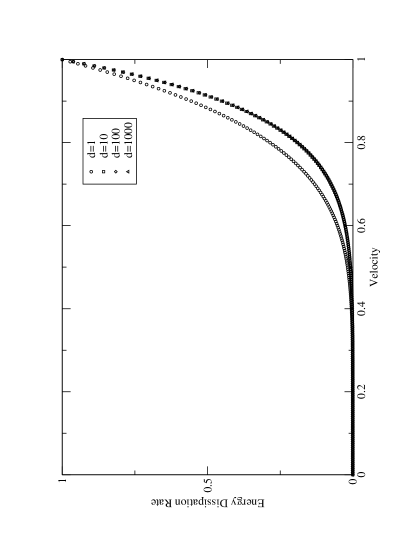
Figure 1: The dissipated energy per unit time for the dipole-like oscillation as a function of the velocity $v$. The velocity is plotted in units of the speed of sound $c_{s}$, and the energy per unit time is scaled by its value for $v=c_{s}$. There are four curves which correspond to the values of amplitude; $d/\xi=1,10,100,1000$.

We estimate the value for critical velocity $v_{c}$ by fitting the curve with the expression $\Gamma\propto v(v-v_{c})$ for small values of $v$. This is based on the standard argument that the condensates will experience the drag force from the impurity, which is proportional to ${\bm{v}}-{\bm{v}_{c}}$. The inner product of this force and the velocity of impurity then gives the rate of dissipated energy in the condensates. The estimated value of the critical velocity for the case $d/\xi=100$ is found as $v_{c}=0.34\;c_{s}$.

IV Energy Dissipation from a Circular Motion

As an another example for periodic motions, we consider a circular motion on the $xy$-plane, which was studied in details in jun2 . The trajectory is specified by two parameters, the radius $R$ and the angular velocity $\Omega$; ${\bm{\zeta}}(t)=(R\cos\Omega t,R\sin\Omega t,0).$ Following the same calculation methods carried out for the previous section, the formula for the dissipated energy per unit time from the circular motion is

$$\Gamma=\sum_{\ell=1}^{\infty}\Gamma_{0}\frac{\ell(k_{\ell}\xi)^{2}}{1+(k_{\ell}\xi)^{2}}\sum_{j=0}^{\infty}{\rm J}_{2j+2\ell+1}(2k_{\ell}R),$$ (26)

where $\Gamma_{0}=n\lambda^{2}M\Omega/(2\pi\hbar^{2}R)$, and the discrete wave number $k_{\ell}$ is given by eq. (25). Note that in the circular motion case, the velocity of the impurity is given by $v=R\Omega$ instead.

We plot the the dissipated energy per unit time in FIG. 2 in the same manner as FIG. 1. The critical velocity for the circular motion is estimated from the graph as $v_{c}=0.43\;c_{s}$. This value is slightly bigger than the case of the dipole oscillation.

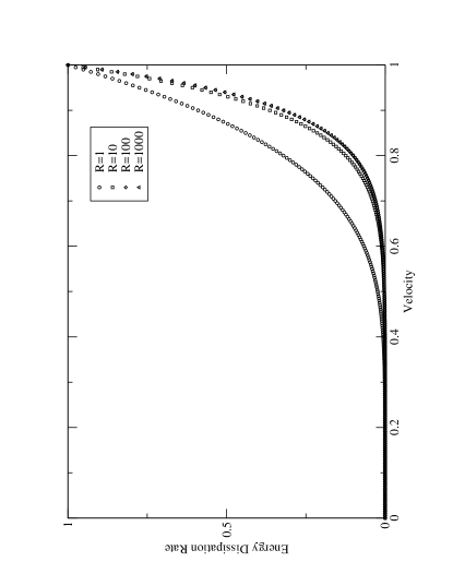
Figure 2: The dissipated energy per unit time for the circular motion as a function of the velocity $v$. The same convention for the units of energy per unit time and the velocity is used as in FIG. 1.

For a comparison, we also plot two cases in FIG. 3 for the value $d/\xi=100$ and $R/\xi=100$. The units of the dissipated energy per unit time in FIG. 3 is $\gamma_{0}=n\lambda^{2}/(2\hbar\xi^{3})$. Two curves show the similarity between two cases. Although we cannot make one to one corresponding for the velocities of two cases, the circular motion has more energy dissipation in general.

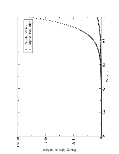
Figure 3: The dissipated energy per unit time for two examples for the amplitude $d/\xi=100$ and the rotation radius $R/\xi=100$. The energy per unit time is in units of $\gamma_{0}=n\lambda^{2}/(2\hbar\xi^{3})$.

V Conclusions and Outlook

We have shown that finite energy dissipation from the periodic motions of impurity can take place even below the Landau critical velocity in the homogeneous BEC. We have found the critical velocities $v_{c}$ for the dipole-like oscillation and the circular motion as $0.34;c_{s}$ and $0.43\;c_{s}$ respectively. Our result qualitatively agrees with the experimental observations of Ref. mit1 ; mit2 ; mit3 . The differences arise from the fact that there are many other factors as pointed out in previous studies jackson ; fedichev ; ref , as well as several simplifications in our model and calculations. It is, therefore, necessary to extend to our model to the case for BECs with trapping potentials at finite temperature to see whether our model yields better agreement or not.

The result present suggest that the landau criterion be reexamined even in the absence of quantized vortices for the homogeneous system. A simple physical argument is that the original Landau’s argument cannot be applied to the case where impurities move under the acceleration. This is because the Galilean invariance fails if there is an acceleration between two coordinates systems. As a related issue, the phenomenon of Cherenkov-like radiation in BECs was studied for an impurity moving with a constant velocity, where the critical velocity for a radiation was found to be exactly same as the Landau critical velocity kovrizhin ; astracharchik ; jun1 ; jun2 .

In this paper we also evaluate the dissipated energy from the circular motion of impurity. A trajectory of the circular motion in BECs is in principle experimentally realizable in current experimental technics. The studies of impurities under the circular motion in BECs may give us further understanding of the coherent properties of condensates and the phenomenon of superfluidities in BECs.

- (1) L. D. Landau, J. Phys. (Moscow) 5, 71 (1941).
- (2) R. P.Feynman, Progress in Low Temperature Physics ed. by C. J. Gorter, Vol. I, Chap. II (North-Holland, Amsterdam 1955).
- (3) N. N. Bogoliubov, J. Phys. (Moscow) 11, 23 (1947).
- (4) M. H. Anderson et al, Science 269, 198 (1995); C. C. Bradley et al, Phys. Rev. Lett. 75, 1687 (1995); K. B. Davis et al, Phys. Rev. Lett. 75, 3969 (1995).
- (5) For a review on BECs, e.g., F. Dalfovo et al, Rev. Mod. Phys. 71, 463 (1999).
- (6) For a review on the Bogoliubov model, V. Zagrebnov and J. -B. Bru, Phys. Rep. 350, 291 (2000).
- (7) C. Raman et al, Phys. Rev. Lett. 83, 2502 (1999).
- (8) R. Onofrio et al, Phys. Rev. Lett. 85, 2228 (2000).
- (9) C. Raman et al, J. Low Temp. Phys. 122, 99 (2001).
- (10) B. Jackson et al, Phys. Rev. A 61, 051603(R) (2000).
- (11) P. O. Fedichev and G. V. Shyyapnikov, Phys. Rev. A 63, 045601 (2001).
- (12) There have been many theoretical works related MIT experiments, see for instance potting ; montina ; mazets ; astracharchik ; pomeau and references therein.
- (13) S. Pötting et al, Phys. Rev. A 64, 023604 (2001).
- (14) A. Montina, Phys. Rev. A 66, 023609 (2002).
- (15) I. E. Mazets, presented at the 7th Intl. Workshop on Atom Optics and Interferometry, Lunteren, Netherlands, Sept.28-Oct.2, 2002; cond-mat/0205235.
- (16) G. E. Astrakharchik and L. P. Pitaevskii, Phys. Rev. A 70, 013608 (2004).
- (17) D. C. Roberet and Y. Pomeau, Phys. Rev. Lett. 95, 145303 (2005).
- (18) P. O. Mazur and J. Suzuki, unpublished (2003).
- (19) J. Suzuki, submitted; cond-mat/0407714.
- (20) J. Suzuki, in preparation; gr-qc/0504141.
- (21) There are several proposals for the number conserving treatment for BEC girardeau ; gardiner ; castin . We follow the one used in refs. girardeau .
- (22) M. D. Girardeau and R. Arnowitt, Phys. Rev. 113, 755 (1959); M. D. Girardeau, Phys. Rev. A 58, 775 (1998).
- (23) C. W. Gardiner, Phys. Rev. A 56, 1414 (1997).
- (24) Y. Castin and R. Dum, Phys. Rev. A 57, 3008 (1998).
- (25) D. L. Kovrizhin and L. A. Maksimov, Phys. Lett. A 282, 421 (2001).