Computation of current-voltage characteristics of weak links

Simplified model for current-voltage characteristics of weak links is suggested. It is based on approach which considers Andreev reflections as responsible for the dissipative current through the metallic Josephson junction. The model allows to calculate current-voltage characteristics of weak links (superconductor - normal metal - superconductor junctions, microbridges, superconducting nanowires) for different thicknesses of the normal layer at different temperatures. The current-voltage characteristics of tin microbridges at different temperatures were computed.

1 Introduction

Superconductor – normal metal – superconductor (SNS) junctions have the current-voltage characteristics (CVCs) with the rich peculiarities. Given certain parameters of junction, CVCs of SNS junctions demonstrate the current peak at the small voltage, the excess current, the subgarmonic gap structure and the negative differential resistance at low bias voltage. Such nonlinear CVCs make SNS junctions to be promising for application to low-noise mixers in submillimetre-wave region [1, 2], switcher [3] or nanologic circuits [4].

Description of CVCs of SNS junctions was subject of many articles and there were recognized key role of multiple Andreev reflections at NS interfaces [5, 6, 7, 8, 9, 10].

The main features of CVCs enumerated above are successfully described by Kümmel - Gunsenheimer - Nicolsky theory (KGN) [7] where time dependent Bogoliubov - de Gennes equations are solved and wave packets of the nonequilibrium electrons and holes are considered. KGN theory is applicable for relatively thick and clean weak links where the normal metal layer N has the thickness $2a$ larger than the coherence length of superconductor and the inelastic mean free path $l$ larger than $2a$. Simplified model in frame of KGN theory was developed by L.A.A. Pereira and R. Nicolsky [11]. This model is relevant for the weak links with thin superconducting banks S. The contribution of the scattering states [7] is omitted in [11].

KGN and Pereira - Nicolsky model were applied earlier to describe the experimental CVCs [12, 13, 14, 15, 16, 17]. Experience of the applications demonstrates that oversimplified Pereira - Nicolsky model gives only qualitative description. New simple modification of KGN theory is proposed in this article. It is shown that CVCs of SNS junctions can be computed without the all complex Ansatz of KGN theory. I hope it will lead to more extensive using of the KGN based approach to the calculation of weak link characteristics than it was earlier [12, 13, 4, 14, 15, 16, 17].

2 Current-voltage characteristics

2.1 Model

Let us consider a voltage-biased SNS junction with a constant electric field which is in negative z direction perpendicular to the NS interfaces and exists in the N layer only (Fig. 1). The normal layer has the thickness $2a$. The thickness of the superconducting bank is $D-a>>2a$.

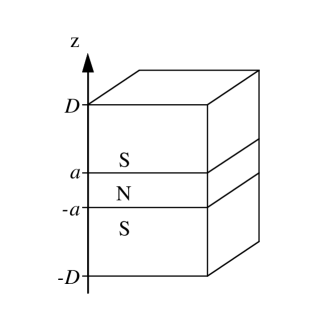
Figure 1: SNS junction modelled.

Accordingly KGN [7] the expression for CVC of SNS junction with thick superconducting banks ($D-a>>2a$) can be written as following:

$$I(V)=\frac{e\hbar}{2am^{\ast}}\sum\limits_{n=1}^{\infty}{\exp\left({-\frac{2a}{l}n}\right)}\qquad\qquad\qquad\qquad\qquad\qquad\qquad\qquad\qquad\$$

$$\int\limits_{-\Delta+neV}^{\Delta+eV}dE\>\sum\limits_{r}g_{r}\left(E\right)P_{N}\left(E\right)k_{zF}\tanh\left({\frac{E}{k_{b}T}}\right)\qquad\quad$$

$$+\frac{V}{R_{N}}\,,\quad$$ (1)

where $m^{\ast}$ is the effective mass of electron, $g_{r}(E)$ is the two dimensional density of states, $P_{N}(E)$ is the probability of finding of the quasiparticles with the energy $E$ in the N region of the thickness $2a$, $l$ is the inelastic mean free path and $R_{N}$ is the resistance of the N region, $\Delta$ is the value of energy gap of superconductor at the temperature $T$, $k_{zF}$ is the z component of Fermi wave vector of quasiparticles, $n$ is the number of Andreev reflections which quasiparticles undergo before they move out of the pair potential well.

Eq.(2.1) is for the time averaged current that includes the voltage dependence only within the integral limits.

2.2 Density of states

To operate on Eq.(2.1) one should calculate the density of states [18]:

$$g_{r}(E)=\frac{A}{\pi}\sum\limits_{r}k_{zF,r}\left|{\frac{dE}{dk_{zF}}}\right|^{-1}_{k_{zF,r}},$$ (2)

where $A$ is the normal layer area, $k_{zF,r}$ defines the value of $k_{zF}$ for which $E_{r}=E$.

The energy spectrum $E_{r}(k_{zF})$ consists of the spatially quantized bound states and the quasicontinuum scattering states. The energy eigenvalue equation for the spatially quantized bound Andreev states [7] is transcendental and calculated numerically only:

$$E_{r}\left({k_{zF}}\right)=\frac{\hbar^{2}k_{zF}}{2am^{\ast}}\left({r\pi+\arccos\frac{E_{r}}{\Delta}}\right),$$ (3)

where $r$ = 0,1,2,…

Let us simplify Eq.(3). The expansion of arccos($E_{r}/\Delta)$ in (3) to Taylor series $(\pi/2-E_{r}/\Delta$ +…) up to second term and subsequent expressing of $E_{r}(k_{zF})$ are executed:

$$E_{r}\left({k_{zF}}\right)\approx\frac{\hbar^{2}k_{zF}}{2am^{\ast}}\pi\left({r+\textstyle{1\over 2}}\right)/\left({1+\\ \frac{\hbar^{2}k_{zF}}{2am^{\ast}\Delta}}\right)$$ (4)

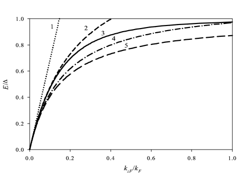
Figure 2: Energy of the bound Andreev state with $r=0$; $2a=5000$ Å; $\Delta=0.57$ meV; $k_{F}=1.62$ Å^-1. 1) Eq.(5), $C=0$; 2) Eq.(5), $C=1$; 3) the exact solution of Eq.(3); 4) Eq.(5), $C=\pi/2(1-am^{\ast}\Delta/\hbar^{2}k_{F})$; 5) Eq.(5), $C=\pi/2$.

Dependence $E_{r}(k_{zF})$ (4) (curve 2) and the numerical solution of Eq.(3) (curve 3) are shown in Fig. 2. The better agreement with the numerical solution of Eq.(3) is attained by insertion of the correcting multiplier $C$ before $\hbar^{2}k_{zF}/2am^{\ast}\Delta$ in Eq.(4):

$$E_{r}\left({k_{zF}}\right)\approx\frac{\hbar^{2}k_{zF}}{2am^{\ast}}\pi\left({r+\textstyle{1\over 2}}\right)/\left({1+C\frac{\hbar^{2}k_{zF}}{2am^{\ast}\Delta}}\right)$$ (5)

If $C=0$ then the spectrum of Pereira - Nicolsky model is reproduced (curve 1, Fig. 2). R. Kümmel used Eq.(5) with $C=\pi/2$ [19] for approximated calculation of the energy spectrum (curve 5, Fig. 2). I suggest the variable multiplier $C=\pi/2(1-am^{\ast}\Delta/\hbar^{2}k_{F})$ for $C>1$ and $C=1$ otherwise. Such choice of $C$ provides a good agreement of Eq.(5) (curve 4, Fig. 2) with the numerical solution of Eq.(3) for different relation of $a,m^{\ast},\Delta,k_{F}$.

The density of the bound states with (5) becomes

$$g_{r}\left(E\right)=\frac{A}{\pi}\left({\frac{2m^{\ast}a}{\hbar^{2}}}\right)^{2}\sum\limits_{r}{\frac{E}{\pi^{2}\left({r+\textstyle{1\over 2}}\right)^{2}\left({1-C\frac{E}{\pi\left({r+\textstyle{1\over 2}}\right)\Delta}}\right)^{3}}}$$ (6)

For quasiparticles from the quasicontinuum states the energy spectrum is approximated by the continuous BCS spectrum of a homogeneous superconductor [7, 18]:

$$E(k_{zF})=\sqrt{\left(\frac{\hbar^{2}}{2m^{\ast}}\left(k_{F}^{2}-k_{zF}^{2}\right)\right)^{2}+{\Delta^{*}}^{2}}$$ (7)

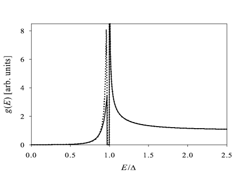
Figure 3: Density of states $g(E)$ of an SNS junction with thick superconducting banks resulted by [18] (dotted line) and $g(E)$ calculated by Eq.(5) with $C=\pi/2(1-am^{\ast}\Delta/\hbar^{2}k_{F})$ (solid line). $D=70000$ Å; $2a=5000$ Å; $T_{c}=3.77$ K; $k_{F}=1.62$ Å^-1.

In the case of SNS junction with thick superconducting banks the effective energy gap $\Delta^{*}$ equals $\Delta$. The density of the quasicontinuum scattering states is

$$g(E)=\frac{A}{\pi^{2}}\frac{2m^{\ast}}{\hbar^{2}}k_{F}D\frac{E}{\sqrt{E^{2}-\Delta^{2}}}$$ (8)

The density of states resulted is shown in Fig. 3.

2.3 Current density

The probability $P_{N}(E)$ of finding of the quasiparticles with the energy $E$ in the N region is given by Eq.(2.19) of [7]:

$$P_{N}(E)=\frac{2a}{2a+2\lambda}$$ (9)

with the penetration depth $\lambda=\frac{\hbar^{2}}{m^{\ast}}\frac{k_{zF}}{\sqrt{\Delta^{2}-E^{2}}}$ for $E<\Delta$, $\lambda<D-a$ and $\lambda=D-a$ otherwise.

For the quasiparticles from the scattering states $P_{N}(E)=2a/2D$. Let us accept for the sake of simplicity $\lambda>>a$ and therefore $P_{N}(E)=2a/2\lambda$ for the bound states.

The current density of quasiparticles from the bound states is resulted with (6):

$$j_{bs}(V)=\frac{e{m^{\ast}}^{2}a^{2}}{2\pi^{3}\hbar^{5}}\sum\limits_{n}\exp\left({-\frac{2a}{l}n}\right)\qquad\qquad\qquad\qquad\qquad\qquad\qquad$$

$$\int\limits_{-\Delta+neV}^{\Delta}{dE\sum\limits_{r}{\frac{\left|E\right|\sqrt{\Delta^{2}-E^{2}}}{\left({r+\textstyle{1\over 2}}\right)\left({1-C\frac{\left|E\right|}{\pi\Delta\left({r+\textstyle{1\over 2}}\right)}}\right)^{3}}}\tanh\left(\frac{E}{2k_{B}T}\right)}$$ (10)

With using (8) the current density of quasiparticles from the quasicontinuum states is resulted:

$$j_{ss}(V)=\frac{e}{4\pi^{2}\hbar}k_{F}\sum\limits_{n}\exp\left({-\frac{2a}{l}n}\right)\qquad\qquad\qquad\qquad\qquad\qquad\qquad$$

$$\int\limits_{E_{1}}^{\Delta+eV}dE\frac{E\sqrt{k_{F}^{2}-\frac{2m^{\ast}}{\hbar^{2}}\sqrt{E^{2}-\Delta^{2}}}}{\sqrt{E^{2}-\Delta^{2}}}\tanh\left(\frac{E}{2k_{B}T}\right)$$ (11)

Here and further $E_{1}$ = $-\Delta+neV$ for $-\Delta+neV\geq\Delta$ and $E_{1}=\Delta$ otherwise.

Neglecting the small term I have

$$j_{ss}(V)=\frac{e}{4\pi^{2}\hbar}{k_{F}}^{2}\sum\limits_{n}{\exp\left({-\frac{2a}{l}n}\right)\int\limits_{E_{1}}^{\Delta+eV}{dE\frac{E\tanh\left({E/2k_{B}T}\right)}{\sqrt{E^{2}-\Delta^{2}}}}}$$ (12)

If $eV>>k_{B}T$, $\Delta$ the integral in (12) can be transformed and the excess current density is resulted:

$$j_{ex}(V)=\frac{e}{2\pi^{2}\hbar}{k_{F}}^{2}\Delta\tanh\left(\frac{eV}{2k_{B}T}\right)\exp\left(-\frac{2a}{l}\right)$$ (13)

This excess current density is the same as one in KGN (Eq.(4.12) in [7]).

Note that $j_{bs}(V)$ dependence does not change practically if the second summation in (2.3) is interrupted at $r=0$. Therefore the total current density is

$$j(V)=\sum\limits_{n}\exp\left({-\frac{2a}{l}n}\right)\Biggl{\{}\frac{2e{m^{\ast}}^{2}a^{2}}{\pi^{3}\hbar^{5}}\int\limits_{-\Delta+neV}^{\Delta}dE{\frac{\left|E\right|\sqrt{\Delta^{2}-E^{2}}}{\left(1-C\frac{2\left|E\right|}{\pi\Delta}\right)^{3}}}\tanh{\left(\frac{E}{2k_{B}T}\right)}$$

$$+\frac{e{k_{F}}^{2}}{4\pi^{2}\hbar}\int\limits_{E_{1}}^{\Delta+eV}dE\frac{E}{\sqrt{E^{2}-\Delta^{2}}}\tanh{\left(\frac{E}{2k_{B}T}\right)}\Biggr{\}}+\frac{V}{R_{N}A}\qquad\qquad$$ (14)

$C=\pi/2(1-am^{\ast}\Delta/\hbar^{2}k_{F})$ for $C>1$ and $C=1$ otherwise; $E_{1}$ = $-\Delta+neV$ for $-\Delta+neV\geq\Delta$ and $E_{1}=\Delta$ otherwise.

Eq.(2.3) is the main result of this simplified model. The model allows to calculate CVCs of weak links for different thicknesses of the normal layer at different temperatures. The subgarmonic gap structure, the excess current and the current peak at the small voltage are reproduced on CVCs.

2.4 Comparison with experimental current-voltage characteristics

The model was used to compute two sets of CVCs of tin microbridges. These detailed measurements of the current biased CVCs were performed by V.N. Gubankov, V.P. Kosheletz, G.A. Ovsyannikov in 1977-1981 [20, 21] (Fig. 4) and M. Octavio, W.J. Skocpol, M. Tinkham in 1978 [22] (Fig. 5). Both sets of CVCs have the similar peculiarities: the subgarmonic gap structure, the current peak at the small voltage and the excess current.

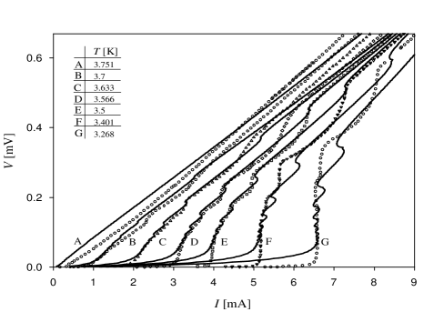
Figure 4: The current-voltage characteristic of Sn microbridges. Experiment [21] (points) and calculations (solid lines).

Comparison of the computed $I(V)$ curves and the experimental $V$ vs. $I$ dependencies displays satisfactory agreement at temperatures smaller than $0.99T_{c}$. Presented in Fig. 4 and Fig. 5 curves were calculated with the reasonable parameters: the critical temperature, the energy gap at zero temperature, the Fermi wave vector of Sn ($T_{c}=3.77$ K, $\Delta_{0}=0.57$ meV, $k_{F}=1.62$ Å^-1). The length of microbridges $2a$ is 5000 Å and $l=15a$. The BCS dependence of $\Delta$ on $T$ was used.

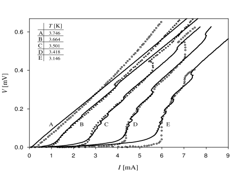
Figure 5: The current-voltage characteristic of Sn microbridges. Experiment [22] (points) and calculations (solid lines).

The high voltages regions on experimental CVCs are close by the computed curves at higher temperatures. It is possibly reasoned by selfheating occurred at high voltages in these experiments [21, 22]. Some discrepancy of the computed curves and the experimental points at low voltages is because there were the current-biased CVCs in experiments instead voltage-biased one. Agreement of the model and the experimental CVCs disappears at temperatures near $T_{c}$: the calculated current peak and the excess current is smaller than corresponding experimental currents (e.g. CVCs at 3.751 K in Fig. 4 and at 3.746 K in Fig.5).

3 Conclusion

Simplified model for calculation of current-voltage characteristics of the weak links (SNS junctions, microbridges, superconducting nanowires) was developed. This model makes the KGN approach [7] more convenient for description of experiments. The model was applied for computation of the current-voltage characteristics of tin microbridges at different temperatures.

References

- [1] Y.A. Gorelov, L.A.A. Pereira, A.M. Luiz, R. Nicolsky. Physica C 282-287, 2491 (1997).
- [2] T. Matsui, H. Ohta. Supercond. Sci. Technol. 12, 859 (1999).
- [3] A.G. Mamalis, D.M. Gokhfeld, S.V. Militsyn, M.I. Petrov, D.A. Balaev, K.A. Shaihutdinov, S.G. Ovchinnikov, V.I. Kirko, I.N. Vottea. Journ. of Materials Processing Technology 161, 42 (2005).
- [4] C.H. Hu, J.F. Jiang, Q.Y. Cai. Supercond. Sci. Technol. 15, 330 (2002).
- [5] T.M. Klapwijk, G.E. Blonder, M. Tinkham. Physica B 109&110, 1657 (1982).
- [6] K. Flensberg, J. Bindslev Hansen, M. Octavio. Phys. Rev. B 38, 8707 (1988).
- [7] R. Kümmel, U. Gunsenheimer, R. Nicolsky. Phys. Rev. B 42, 3992 (1990).
- [8] U. Gunsenheimer, A.D. Zaikin. Phys. Rev. B 50, 6317 (1994).
- [9] E.N. Bratus’, V.S. Shumeiko, E.V. Bezuglyi, G. Wendin. Phys. Rev. B 55, 12666 (1997).
- [10] A. Bardas, D. Averin. Phys. Rev. B 56, 8518 (1997).
- [11] L.A.A. Pereira, R. Nicolsky. Physica C 282-287, 2411 (1997).
- [12] L.A.A. Pereira, A.M. Luiz, R. Nicolsky. Physica C 282-287, 1529 (1997).
- [13] M.I. Petrov, D.A. Balaev, D.M. Gohfeld, S.V. Ospishchev, K.A. Shaihutdinov, K.S. Aleksandrov. Physica C 314, 51 (1999).
- [14] M.I. Petrov, D.A. Balaev, D.M. Gokhfeld, K.A. Shaikhutdinov, K.S. Aleksandrov. Fiz. Tverd. Tela 44, 1179 (2002) [Phys. Solid State 44, 1229 (2002)].
- [15] M.I. Petrov, D.A. Balaev, D.M. Gokhfeld, K.A. Shaikhutdinov. Fiz. Tverd. Tela 45, 1164 (2003) [Phys. Solid State 45, 1219 (2003)].
- [16] M.I. Petrov, D.M. Gokhfeld, D.A. Balaev, K.A. Shaihutdinov, R. Kümmel. Physica C 408, 620 (2004).
- [17] D.M. Gokhfeld, D.A. Balaev, K.A. Shaykhutdinov, S.I. Popkov, M.I. Petrov. cond-mat/0410112 (2004).
- [18] H.Plehn, U. Gunsenheimer, R. Kümmel. Journ. Low Temp. Phys. 83, 71 (1991).
- [19] R. Kümmel. Private communications.
- [20] V.N. Gubankov, V.P. Kosheletz, G.A. Ovsyannikov. Journ. Exp. i Teoretich. Fiziki 73, 1435 (1977).
- [21] V.N. Gubankov, V.P. Kosheletz, G.A. Ovsyannikov. Fizika Nizkikh Temperatur 7, 277 (1981).
- [22] M. Octavio, W.J. Skocpol, M. Tinkham. Phys. Rev. B 17, 159 (1978).