Energy entanglement in normal metal-superconducting forks

Abstract

The possibility for detecting energy entanglement in normal metal–superconductor junctions is examined. For the first time we proved that two electrons in a NS structure originating from the same Cooper pair are entangled in the energy subspace. This work follows previous works where spin entanglement was studied in similar circuits. The device consists of a superconducting beam splitter connected to two electronic Mach-Zehnder interferometers. In each arms of the interferometers, energies are filtered with coherent quantum dots. In contrast to previous studies of zero-frequency cross-correlations of electrical currents for this system, attention is drawn to finite-time measurements. This allows to observe two-particle interference for particles with different energies above and below Fermi level. Entanglement is first characterized via the concurrence for the two-particle spatial density matrix. Next, we formulate the Bell inequality, which is written in terms of finite-time noise correlators, and thereby we find a specific set of parameters for which entanglement can be detected.

I Introduction

Entanglement is the building block of quantum information processing schemes bouw . In recent years, it has generated considerable excitement in the mesoscopic physics and nanophysics community. Over the years, electronic analogs of optical setups have been conceived in order to probe entanglement between electrons. In the context of electron transport, entanglement was first described theoretically lesovik_martin_blatter ; recher_sukhorukov_loss in forked normal metal-superconductor devices revealing positive noise cross-correlations torres_martin . Then entanglement in such devices was quantified via the Bell inequality test chtchelkatchev .

In all these schemes a superconductor injects Cooper pairs in two metallic arms, or in quantum dots connected to leads. When two electrons are emitted from the superconductor, they either get into the same lead or in opposite leads. The resulting zero frequency noise correlations between the two normal arms will have a tendency to be negative in the former process due to the partition noise of Cooper pairs. The latter process, also called crossed-Andreev process, is the source of entanglement, and leads to positive noise correlations. Indeed, the Cooper pair is transmitted as a singlet state, and it is entangled both in spin and in energy.

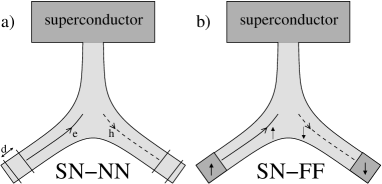
Figure 1: a) Normal metal-superconducting fork with energy filters selecting electron ($+E$) on the left side and selecting holes ($-E$) on the right side. b) Same fork, but this time with spin filters, leaving the possibility of energy entanglement as both electrons and holes (with a definite spin for each side) can propagate in both branches.

The detection of spin entanglement has been addressed on several occasions for ideal devices burkard_loss ; saraga , and with the assumption that parasitic effects are present sauret_martin_feinberg . In optics, a standard test for studying the degree of entanglement of two photons is to perform a Bell/Clauser Horne inequality test, in a coincidence measurement. This test allows to probe the non-local nature of quantum mechanics: are the two particles in an entangled state? In contrast, in condensed matter physics, experiments are often performed in a stationary state, with constant currents flowing at the output. Nevertheless, in Ref. chtchelkatchev it was shown that a Bell inequality test kawabata can be expressed in terms of zero frequency noise cross-correlations at the output. Subsequently, similar Bell inequality tests were proposed for orbital entanglement in a superconducting setup orbital_entanglement , in normal metal devices Entanglement3 ; Entanglement4 , and in Quantum Hall systems beenakker ; buttiker .

Ref. lesovik_martin_blatter proposed that some constraints should be imposed on a plain superconducting-normal metal fork torres_martin in order to probe entanglement. Energy filters where added on each side [Fig. 1(a)], selecting positive/negative energies depending on the side. An incoming hole thus could only be reflected as an electron in the opposite branch, yet the spin degree of freedom was untouched. Energy entanglement was also proposed lesovik_martin_blatter using spin filters instead of energy filters [Fig. 1(b)]. Except for the characterization of positive noise correlations which constitutes a symptom of entanglement, so far no quantitative test of this entanglement has been reached.

Recent advances in quantum optic experiments on momentum-phase entanglement rarity led to experimental realization of such techniques as two-particle teleportation teleportation , the purification protocol for polarization entangled state purification and the full Bell-state analysis bell_analiser . All of the above provide additional motivation for us to reexamine the question of energy entanglement.

The purpose of this work is to explain how energy entanglement can be detected in normal metal-superconducting forks. Although the setup which we propose is built from elementary building blocks of mesoscopic physics, it is rather elaborate. We thus emphasize that our main goal is to show whether energy entanglement detection is plausible from a theoretical standpoint.

The paper is organized as follow: Sec. 2 gives a basic description of the setup, which is composed of a superconducting fork connected to two Mach-Zehnder (MZ) interferometers. Sec. 3 and 5 describe the calculation of the two-particle density matrix and electrical current cross-correlations in the context of scattering theory for this normal metal-superconductor setup. Sec. 4 describes the entanglement characterization via the concurrence of the density matrix. Sec. 6 develops the Bell inequality analysis in terms of electrical currents.

II Description of the setup

We now present a setup (Fig. 2), which is able to test energy entanglement via the violation of Bell inequalities. We use a normal-metal fork connected to a superconductor. The leads connected to the arms of this fork are assumed to have quasiparticle mean free path larger than the size of the setup: in this ideal version of the setup, backscattering is absent. A possibility would be to use electrostatically defined quantum wires on semiconductor heterostructures, assuming that the interface between the two dimensional electron gas and the superconductor can be controlled. The two leads connected to the injection fork (center of Fig. 2) are each attached to two other forks (left and right of Fig. 2), which filter the particles according to their positive/negative energy, measured with respect to the chemical potential of the superconductor. This energy filtering can in principle be realized via a double barrier structure forming an electronic Fabry-Perot interferometer. An example of such a filter was demonstrated in a ”which path detection” experiment at the Weizmann Institute Umansky ) where one arm of the devices contained a coherent quantum dot.

Next, the two forks on the right and on the left are reconnected, forming MZ interferometers. The paths on each arm of such interferometers have equal length, and the two beam splitters are assumed to be symmetrical. Later on in this paper, we shall consider the measurements of current cross-correlations performed between different contacts $A_{1}$, $A_{2}$, $B_{3}$ and $B_{4}$ of these two interferometers. Note that, in this suggested geometry of the setup, there is no absolute need for spin-filters, contrarily to what was suggested in Ref. lesovik_martin_blatter, and illustrated in Fig. 1(b). As we shall see below, if the interface between the injecting fork and the superconductor is opaque, the two constituent electrons of a Cooper pair are split between the right and left side and the cross correlation signal is positive, as in a photon coincidence measurement.

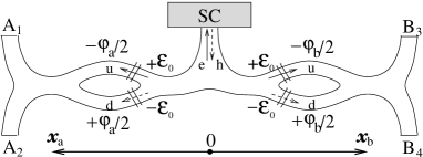
Figure 2: Setup for measuring energy entanglement from a normal metal-superconducting fork. The superconductor emits Cooper pairs in the ballistic region. The electrons from a pair are then spit on the first fork. Then the particles are filtered according to their energy. The amplitudes for particles with energies above and below Fermi level are combined at the last beam splitter, in close analogy with the optical setup rarity .

The idea of this experiment is that two electrons, which originate from a Cooper pair in the superconductor, once on the normal metal side, have energies which are symmetric with respect to the chemical potential of the superconductor. In principle they can be filtered in a way that an electron with energy above this Fermi level always gets into the upper arms of the interferometers (energy $+\epsilon_{0}$, leads $u_{A}$ and $u_{B}$ in Fig. 2) or it gets into the lower arms of interferometers otherwise (energy $-\epsilon_{0}$, leads $d_{A}$ and $d_{B}$ in Fig. 2). That is, two electrons being split at the injection superconducting fork (center of Fig. 2) always end up into the right upper and the left lower arms of the interferometers or into the right lower and the left upper ones.

This situation is very similar to the phase-momentum entanglement in quantum optics. Indeed, an experimental non-locality test for photons was achieved by Rarity and Tapster using two MZ interferometers rarity . Two photons with different wave lengths were generated during a down-conversion process, and subsequent recombination of the beams allowed to perform a correlation measurement. We find that this quantum optics experiment can be translated for and applied to electronic devices. As we shall see, in our condensed matter analog, which uses charged particles, the Bell inequality violation can be tuned by varying the magnetic fluxes within interferometers (electrons gain extra phases $e^{\pm i\varphi_{a}/2}$ and $e^{\pm i\varphi_{b}/2}$ in the lower (upper) arms of the interferometers).

In the quantum optics experiment rarity , the momentum direction of the down-converted photons allowed to separate the photons and to let them recombine at the beam splitters, provided that a single beam splitter can be reached only by photons with equal frequencies. This property is essential for the two-particle interference. In our proposal the particles, which are reaching the last beam splitters (recombination of the beams) along different paths, have different energies, so it is in principle possible to achieve ”which path” information and therefore to destroy the interference. We propose to use measurements on short enough time scales so that it is not possible to resolve the energy of the particle (energy/time Heisenberg principle). We claim that the two-particle interference and the non-local properties of quantum mechanics can be detected in this ideal setup.

III Calculation of the density matrix

In order to analyze the properties of the injected electrons, we calculate the two-particle density matrix for quasiparticles caught right after energy filters (in leads $u_{A}$, $d_{A}$ and $u_{B}$, $d_{B}$):

$$g(\vec{\sigma},\vec{x})=Tr\left[\hat{\rho}\hat{\Psi}_{\sigma_{1}^{\prime}}^{\dagger}(x_{i^{\prime}})\hat{\Psi}_{\sigma_{2}^{\prime}}^{\dagger}(x_{j^{\prime}})\hat{\Psi}_{\sigma_{2}}(x_{j})\hat{\Psi}_{\sigma_{1}}(x_{i})\right],$$ (1)

here we have written the whole matrix with non-diagonal elements, and the indexes $\sigma$ describe the spins part of density matrix, and orbital indexes $i=u_{A},d_{A}$ and $j=u_{B},d_{B}$ describe the lead there the particle is caught. In practice, only diagonal elements with $x_{i}=x_{i^{\prime}}$ and $x_{j}=x_{j^{\prime}}$ can be measured, but our task is to analyze the amount of entanglement which is implicit in such a matrix, therefore non-diagonal elements play a crucial role.

In our calculations we follow the scattering theory approach developed in Noise1 ; Noise2 , and later applied to NS-systems with Andreev scattering Noise_NS . For background purposes, the reader is referred to the reviews Blanter_Buttiker ; Martin_Review . Here we follow closely the notations of Ref. Noise3, . For simplicity, we consider ballistic quasi one-dimensional quantum wires without backscattering. The transport in this system is governed by the properties of Andreev reflection and normal reflection of electrons and holes. So it is useful to perform Bogoliubov transformation (see Ref. bogolubov_de_gennes, ) for the annihilation operator of a particle at a position $x$ with up/down spin $\sigma=\pm 1$:

$$\hat{\Psi}_{i,\sigma}(x_{i},t_{i})=\frac{1}{\sqrt{2\pi}}\sum_{j,\beta}\int_{0}^{+\infty}dE\left(\frac{u_{ij\beta}(x_{i})}{\sqrt{\hbar v_{e}^{j}(E)}}\hat{c}_{j\beta\sigma}(E,t_{i})-\right.$$

$$~{}~{}~{}~{}~{}~{}~{}~{}~{}~{}~{}~{}~{}~{}~{}~{}\left.-\sigma\frac{v_{ij\beta}^{*}(x_{i})}{\sqrt{\hbar v_{h}^{j}(E)}}\hat{c}_{j\beta-\sigma}^{+}(E,t_{i})\right).$$ (2)

The states $u_{ij\beta}$ or $v_{ij\beta}$ correspond to wave functions of an electron or a hole scattered in lead $i$, due to a quasiparticle of type $\beta=e,h$ incoming from lead $j$. Operators $\hat{c}_{j\beta\sigma}(E)$ and $\hat{c}_{j\beta\sigma}^{+}(E)$ satisfy standard Fermi statistic relations. $v_{e}^{j}(E)=\hbar k_{e}^{j}(E)$ and $v_{h}^{j}(E)=\hbar k_{h}^{j}(E)$ are velocities of electrons and holes in lead $j$.

The evolution of particle states $u_{ij\beta}$ and $v_{ij\beta}$ is described by Bololiubov-de Gennes equations, which can be written as

$$\left(-\frac{\hbar^{2}}{2m}\frac{\partial^{2}}{\partial x^{2}}-\mu_{S}+V(x)\right)u_{ij\beta}(x)$$

$$~{}~{}~{}~{}~{}~{}~{}~{}~{}~{}~{}~{}~{}~{}~{}~{}~{}~{}~{}~{}+\Delta(x)v_{ij\beta}(x)=Eu_{ij\beta}(x),$$ (3a)

$$\left(+\frac{\hbar^{2}}{2m}\frac{\partial^{2}}{\partial x^{2}}+\mu_{S}-V(x)\right)v_{ij\beta}(x)$$

$$~{}~{}~{}~{}~{}~{}~{}~{}~{}~{}~{}~{}~{}~{}~{}~{}~{}~{}~{}~{}+\Delta^{*}(x)u_{ij\beta}(x)=Ev_{ij\beta}(x).$$ (3b)

The pair potential $\Delta(x)$ should be calculated selfconsistently, but, for simplicity, in our calculation it corresponds to the superconducting gap $\Delta$ in the bulk of the superconductor ($x>0$), and it is zero in the normal leads ($x<0$).

In a normal ideal lead $\Delta(x)=0$ and $V(x)=0$, Bogoliubov-de Gennes equations (3a)-(3b) reduce to Schrodinger equation for free electrons and holes. Solutions of form $e^{ik_{e}^{N}x}$ for electrons and $e^{ik_{h}^{N}x}$ for holes are chosen, where $k_{e}^{N}=\sqrt{2m(\mu_{S}+E)}/\hbar$ and $k_{h}^{N}=\sqrt{2m(\mu_{S}-E)}/\hbar$ are wave vectors for electrons and holes.

Electrons and holes that originate from a particle of type $\beta$ in lead $j$ and scattered into lead $i$ are described by:

$$u_{ij\beta}(x_{i})=\delta_{ij}\delta_{e\beta}e^{+ik_{e}^{N}x_{i}}+S_{ij}^{e\beta}\sqrt{\frac{k_{\beta}^{j}}{k_{e}^{N}}}e^{-ik_{e}^{N}x_{i}},$$ (4a)

$$v_{ij\beta}(x_{i})=\delta_{ij}\delta_{h\beta}e^{-ik_{h}^{N}x_{i}}+S_{ij}^{h\beta}\sqrt{\frac{k_{\beta}^{j}}{k_{h}^{N}}}e^{+ik_{h}^{N}x_{i}}.$$ (4b)

Here we have the opposite sign for momenta of electrons and holes, which is due to the symmetry of Bogoliubov-de Gennes equations. For simplicity, we introduced a notation $S_{ij}^{\alpha\beta}$ for scattering-matrix element expressing the amplitude of an outgoing particle of type $\alpha$ in lead $i$ due to an incident particle of type $\beta$ in lead $j$. In general, these amplitudes depend on the quasiparticle energies.

We linearize the wave vectors in energy in the exponents, and then take them equal to $k_{F}$ in pre-exponential factors. We substitute all the equations into Eq. (1) and obtain:

$$\;\;\;\;\;\;\;\;g(\vec{\sigma},\vec{x})=\frac{1}{(hv_{F})^{2}}\sum\limits_{k,l,m,n}\int_{0}^{+\infty}\dots\int_{0}^{+\infty}dE_{1}\dots dE_{4}\times$$ (5)

$$\left[\left\langle\hat{c}_{k\sigma_{1}^{\prime}}^{\dagger}(E_{1},t_{i^{\prime}})\hat{c}_{l\sigma_{2}^{\prime}}^{\dagger}(E_{2},t_{j^{\prime}})\hat{c}_{m\sigma_{2}}(E_{3},t_{j})\hat{c}_{n\sigma_{1}}(E_{4},t_{i})\right\rangle u_{i^{\prime}k}^{*}(x_{i^{\prime}})u_{j^{\prime}l}^{*}(x_{j^{\prime}})u_{jm}(x_{j})u_{in}(x_{i})\right.$$ (6)

$$+\left\langle\hat{c}_{k\sigma_{1}^{\prime}}^{\dagger}(E_{1},t_{i^{\prime}})\hat{c}_{l-\sigma_{2}^{\prime}}(E_{2},t_{j^{\prime}})\hat{c}_{m-\sigma_{2}}^{\dagger}(E_{3},t_{j})\hat{c}_{n\sigma_{1}}(E_{4},t_{i})\right\rangle\sigma_{2}^{\prime}\sigma_{2}u_{i^{\prime}k}^{*}(x_{i^{\prime}})v_{j^{\prime}l}(x_{j^{\prime}})v_{jm}^{*}(x_{j})u_{in}(x_{i})$$ (7)

$$+\left\langle\hat{c}_{k\sigma_{1}^{\prime}}^{\dagger}(E_{1},t_{i^{\prime}})\hat{c}_{l-\sigma_{2}^{\prime}}(E_{2},t_{j^{\prime}})\hat{c}_{m\sigma_{2}}(E_{3},t_{j})\hat{c}_{n-\sigma_{1}}^{\dagger}(E_{4},t_{i})\right\rangle\sigma_{2}^{\prime}\sigma_{1}u_{i^{\prime}k}^{*}(x_{i^{\prime}})v_{j^{\prime}l}(x_{j^{\prime}})u_{jm}(x_{j})v_{in}^{*}(x_{i})$$ (8)

$$+\left\langle\hat{c}_{k-\sigma_{1}^{\prime}}(E_{1},t_{i^{\prime}})\hat{c}_{l\sigma_{2}^{\prime}}^{\dagger}(E_{2},t_{j^{\prime}})\hat{c}_{m-\sigma_{2}}^{\dagger}(E_{3},t_{j})\hat{c}_{n\sigma_{1}}(E_{4},t_{i})\right\rangle\sigma_{1}^{\prime}\sigma_{2}v_{i^{\prime}k}(x_{i^{\prime}})u_{j^{\prime}l}^{*}(x_{j^{\prime}})v_{jm}^{*}(x_{j})u_{in}(x_{i})$$ (9)

$$+\left\langle\hat{c}_{k-\sigma_{1}^{\prime}}(E_{1},t_{i^{\prime}})\hat{c}_{l\sigma_{2}^{\prime}}^{\dagger}(E_{2},t_{j^{\prime}})\hat{c}_{m\sigma_{2}}(E_{3},t_{j})\hat{c}_{n-\sigma_{1}}^{\dagger}(E_{4},t_{i})\right\rangle\sigma_{1}^{\prime}\sigma_{1}v_{i^{\prime}k}(x_{i^{\prime}})u_{j^{\prime}l}^{*}(x_{j^{\prime}})u_{jm}(x_{j})v_{in}^{*}(x_{i})$$ (10)

$$\left.+\left\langle\hat{c}_{k-\sigma_{1}^{\prime}}(E_{1},t_{i^{\prime}})\hat{c}_{l-\sigma_{2}^{\prime}}(E_{2},t_{j^{\prime}})\hat{c}_{m-\sigma_{2}}^{\dagger}(E_{3},t_{j})\hat{c}_{n-\sigma_{1}}^{\dagger}(E_{4},t_{i})\right\rangle\sigma_{1}^{\prime}\sigma_{2}^{\prime}\sigma_{2}\sigma_{1}v_{i^{\prime}k}(x_{i^{\prime}})v_{j^{\prime}l}(x_{j^{\prime}})v_{jm}^{*}(x_{j})v_{in}^{*}(x_{i})\right],$$ (11)

here the summation over indexes $k$, $l$, $m$ and $n$ implies a summation over lead indexes and types of particles - $e$ or $h$.

We consider the case where all normal leads are biased with the same voltage $V$. With these assumptions, the density matrix takes the form (see Appendix):

$$g(\vec{\sigma},\vec{x})=\delta_{\sigma_{1}\sigma_{1}^{\prime}}\delta_{\sigma_{2}\sigma_{2}^{\prime}}G_{i^{\prime}i}G_{jj^{\prime}}^{*}-\delta_{\sigma_{1}\sigma_{2}^{\prime}}\delta_{\sigma_{2}\sigma_{1}^{\prime}}G_{i^{\prime}j}G_{ij^{\prime}}^{*}+I_{\sigma_{1}\sigma_{2}}I_{\sigma_{1}^{\prime}\sigma_{2}^{\prime}}F_{i^{\prime}j^{\prime}}F_{ij}^{*},$$ (12)

where we have used a notation for a matrix: $I_{\sigma_{1}\sigma_{2}}=i\hat{\tau}_{y}$ and $\hat{\tau}_{y}$ is a Pauli matrix. We compute this density matrix at locations taken in the leads of the interferometers: $u_{A}$, $d_{A}$, $u_{B}$ and $d_{B}$ (See Fig. 2). We thus define indices $i$ and $i^{\prime}$ which can take the values $u_{A}$ or $d_{A}$ and indexes $j$ and $j^{\prime}$ equal to $u_{B}$ or $d_{B}$. We also use a notation for the two-point correlation functions:

$$G_{ij}(x_{i},x_{j},t_{j}-t_{i})=\frac{1}{hv_{F}}\sum\limits_{k}\int_{-\infty}^{+\infty}dEf_{k}(E)(u_{ik}^{*}(x_{i})u_{jk}(x_{j}))e^{-iE(t_{j}-t_{i})},$$ (13a)

$$F_{ij}(x_{i},x_{j},t_{j}-t_{i})=\frac{1}{hv_{F}}\sum\limits_{k}\int_{-\infty}^{+\infty}dEf_{k}(E)(u_{ik}^{*}(x_{i})v_{jk}(x_{j}))e^{-iE(t_{j}-t_{i})}.$$ (13b)

Up to now, we have not specified the transmission properties of the combined normal metal fork/superconductor plus energy filtering forks. For the parametrization of the beam splitter connected to the superconductor we take a scattering matrix with real amplitudes described in gefen_buttiker :

$$U_{SL_{0}R_{0}}=\left(\begin{array}[]{ccc}-(a+b)&\sqrt{\epsilon}&\sqrt{\epsilon}\\ \sqrt{\epsilon}&a&b\\ \sqrt{\epsilon}&b&a\end{array}\right),$$ (14)

with the free parameter $0\leq\epsilon\leq\frac{1}{2}$ describing the transmission probability between the top lead and the right and left arms. In general, there are two possible choices of parametrization lesovik_martin_blatter : $a=\frac{\sqrt{1-2\epsilon}-1}{2}$, $b=\frac{\sqrt{1-2\epsilon}+1}{2}$, or alternatively $a$ and $b$ can be exchanged. Here we use the first parametrization: it corresponds to a good transmission for electrons (holes) entering from the left lead of the fork and exiting from the right one, and vice versa. We claim that the excess parts of all the correlators are the same if one choses the opposite convention. This unitary matrix (14) is assumed to be the same for electrons and holes, which implies a weak dependence of the scattering matrix on energy. Due to multiple Andreev reflection on $NS$-boundary and a phase shift in the superconducting lead (S), the transmission amplitudes change in an analogous manner to a Fabry-Perot interferometer. Assuming ideal Andreev reflection on the boundary of the superconductor: $r_{SS}^{eh}=r_{SS}^{he}=e^{-i\arccos{\frac{E}{\Delta}}}$, and $e^{-i\eta}=r_{SS}^{eh}e^{-iE\frac{2S}{v_{F}\hbar}}$ one can get

$$A=r_{LL}^{\alpha\alpha}=r_{RR}^{\alpha\alpha}=a-\frac{\epsilon(a+b)e^{-2i\eta}}{1-(a+b)^{2}e^{-2i\eta}},$$ (15a)

$$B=t_{LR}^{\alpha\alpha}=t_{RL}^{\alpha\alpha}=b-\frac{\epsilon(a+b)e^{-2i\eta}}{1-(a+b)^{2}e^{-2i\eta}},$$ (15b)

$$C=r_{LL}^{\alpha\beta}=r_{RR}^{\alpha\beta}=\frac{\epsilon e^{-i\eta}}{1-(a+b)^{2}e^{-2i\eta}},$$ (15c)

$$D=t_{LR}^{\alpha\beta}=t_{RL}^{\alpha\beta}=\frac{\epsilon e^{-i\eta}}{1-(a+b)^{2}e^{-2i\eta}},$$ (15d)

here $A$ and $B$ are reflection and transmission amplitudes for particles of the same type ($\alpha\alpha$) with incident and final lead to the left ($L$) and to the right ($R$) from the fork, and $C$ and $D$ are reflection and transmission amplitudes for the case of changed types of particles ($\alpha\beta$). Although notations $A$, $B$, $C$, $D$ are not used here, they are introduced for later convenience, in Eqs. (35a) and (35b).

The energy filtering forks are chosen “ideal”: electrons with energies above the superconducting chemical potential pass without reflection through the upper arm, while electrons which energy is below this chemical potential go in the lower arm of the fork (left side of Fig. 2). The following transmission amplitudes are thus chosen for the left energy filtering fork:

$$r_{LL}^{ee}(\pm E)=0,$$ (16a)

$$r_{uu}^{ee}(+E)=0, \;\;\;\;r_{uu}^{ee}(-E)=-1,$$ (16b)

$$r_{dd}^{ee}(+E)=+1, \;\;\;\;r_{dd}^{ee}(-E)=0,$$ (16c)

$$t_{uL}^{ee}(+E)=1, \;\;\;\;t_{uL}^{ee}(-E)=0,$$ (16d)

$$t_{dL}^{ee}(+E)=0, \;\;\;\;t_{uL}^{ee}(-E)=-i,$$ (16e)

here the amplitudes for hole type quasiparticles follow from Eq. (63) and the same is correct for the right fork exchanging $L$ on $R$. This is a very simple parametrization, and the only constraint is the unitary conditions. In a real experiment there may be a more complicated dependence on energy leading to imperfections, but this question goes beyond the scope of the paper.

Now the global scattering amplitudes are calculated in a simple way, because of our assumption of no backscattering in the leads. For example:

$$S_{u_{L}d_{L}}^{ee}=r_{uu}^{ee}+t_{uL}^{ee}S_{LL}^{ee}t_{Lu}^{ee}~{}.$$ (17)

These amplitudes allow to calculate the pair correlation functions from the Eqs. (13a) and (13b), and the results may be divided into an equilibrium and an excess part:

$$G_{ij}(x_{i},x_{j},\Delta t_{ij})=G_{ij}^{eq}(x_{ij}^{+},\Delta t_{ij})+G_{ij}^{ex}(\Delta x_{ij},\Delta t_{ij})~{},$$ (18)

the former depends on the sum of coordinates and describes the Fermi correlations within normal leads, the latter depends on the difference of coordinates and describes the particles injected from the superconductor. The most interesting contributions for the discussion below are the excess contributions which dominate at low temperatures ($T\ll eV$):

$$G_{ij}^{ex}= -\delta_{ij}\frac{\epsilon^{2}}{2(1-\epsilon)^{2}}e^{-ik_{F}\Delta x_{ij}}e^{\pm i\frac{eV}{2v_{F}\hbar}(\Delta x_{ij}+\Delta t_{ij})}$$ (19b)

$$\times\frac{\sin{\frac{eV}{2v_{F}\hbar}(\Delta x_{ij}+\Delta t_{ij})}}{\pi(\Delta x_{ij}+\Delta t_{ij})},$$

$$F_{ij}^{ex}= \delta_{i\overline{j}}\frac{\epsilon\sqrt{1-2\epsilon}}{2(1-\epsilon)^{2}}e^{+ik_{F}x_{ij}^{+}}e^{\pm i\frac{eV}{2v_{F}\hbar}(\Delta x_{ij}+\Delta t_{ij})}$$

$$\times\frac{\sin{\frac{eV}{2v_{F}\hbar}(\Delta x_{ij}+\Delta t_{ij})}}{\pi(\Delta x_{ij}+\Delta t_{ij})},$$

where $i=u_{A},d_{A}$ and $i=u_{B},d_{B}$; $\epsilon$ is the scattering parameter of Eq.(14) of the superconducting fork; $\Delta x_{ij}=x_{j}-x_{i}$ and $\Delta t_{ij}=t_{j}-t_{j}$; and $\delta_{ij}$ ($\delta_{i\overline{j}}$) is equal to unity (zero) only if $i$ and $j$ are simultaneously $u$ or $d$.

IV Concurrence for the density matrix

We now turn to the calculation of the concurrence, as defined in the work of Wootters wootters , but adapted to our transport geometry. With the additional assumption of simultaneous measurements (all the times $t_{i}$ in Eq. (19b) are the same) and equal coordinates on the same sides of the setup ($x_{u_{A}}=x_{d_{A}}$ and $x_{u_{B}}=x_{d_{B}}$, up to a the precision $\delta x\ll v_{F}\tau_{V}$) the whole density matrix simplifies to:

$$g(\vec{\sigma},\vec{x})= g_{0}^{2}\left[\delta_{\sigma_{1}\sigma_{1}^{\prime}}\delta_{\sigma_{2}\sigma_{2}^{\prime}}\delta_{i^{\prime}i}\delta_{jj^{\prime}}\right.$$ (20)

$$-\delta_{\sigma_{1}\sigma_{2}^{\prime}}\delta_{\sigma_{2}\sigma_{1}^{\prime}}\delta_{i^{\prime}j}\delta_{ij^{\prime}}e^{\pm i\varphi}g^{2}(\Delta_{x})$$

$$\left.+I_{\sigma_{1}\sigma_{2}}I_{\sigma_{1}^{\prime}\sigma_{2}^{\prime}}\delta_{i^{\prime}\overline{j^{\prime}}}\delta_{i\overline{j}}e^{\pm i\varphi}f^{2}(\Delta_{x})\right],$$

where

$$g_{0}=\frac{\epsilon^{2}}{2(1-\epsilon)^{2}}\frac{eV}{2\pi v_{F}\hbar},\;\;\;\;g(\Delta x)=\frac{\sin{\frac{\Delta x}{2v_{F}\tau_{V}}}}{\frac{\Delta x}{2v_{F}\tau_{V}}},$$ (21)

$$f(\Delta x)=\frac{\sqrt{1-2\epsilon}}{\epsilon}g(\Delta x),$$ (22)

where $\tau_{V}=\hbar/eV$. For $i=j^{\prime}=u$ and $i^{\prime}=j=d$, the parameter $\varphi=\frac{eV}{v_{F}\hbar}\Delta x$ which appear in Eq. (20) is taken with a plus sign, for $i=j^{\prime}=d$ and $i^{\prime}=j=u$ - with a minus sign, and in all other cases it is zero.

The two-particle density matrix describing the spin entangled state of two quasi-particles inside a superconductor has been already studied in Kim for a bulk superconductor. In contrast, our analysis allows to study energy entanglement in a condensed matter setting with normal metal leads, which are essential for the diagnosis of entanglement. Since we are not interested in the spin entanglement here, we trace Eq. (20) over spin degrees of freedom, and we obtain a density matrix which depends only on orbital degrees of freedom:

$$g_{i,j;i^{\prime},j^{\prime}}=Tr_{\sigma}g(\vec{\sigma},\vec{x})=2g_{0}^{2}N\hat{\rho}_{AB}$$ (23)

$$\hat{\rho}_{AB}=\frac{1}{N}\left(\begin{array}[]{cccc}2-g^{2}&0&0&0\\ 0&2+f^{2}&(f^{2}-g^{2})e^{+i\varphi}&0\\ 0&(f^{2}-g^{2})e^{-i\varphi}&2+f^{2}&0\\ 0&0&0&2-g^{2}\end{array}\right),$$ (24)

where the normalization factor $N=8+2f^{2}-2g^{2}$ is chosen so that the trace for this matrix is unity. The parameter $g^{2}\leq 1$. It turns out that the parameter $\varphi=\frac{eV}{v_{F}\hbar}\Delta x$ does not appear in the final result for the entanglement measure.

One of the possible expansions (on the basis of pure states) for such a mixed state may be written in the space of the pseudo-spin $|\uparrow\rangle=|u\rangle$ and $|\downarrow\rangle=|d\rangle$:

$$\hat{\rho}_{AB}=\frac{1}{N}\left[(f^{2}-g^{2})|\Psi^{(+)}\rangle\langle\Psi^{(+)}|+(2-g^{2})\hat{\bf I}\right.$$

$$\;\;\;\;\left.+2g^{2}\left(|\uparrow_{A}\downarrow_{B}\rangle\langle\uparrow_{A}\downarrow_{B}|+|\downarrow_{A}\uparrow_{B}\rangle\langle\downarrow_{A}\uparrow_{B}|\right)\right],$$ (25)

where $\hat{\bf I}$ - the unity matrix, and the only entangled term in the sum corresponds to the state:

$$|\Psi^{(+)}\rangle=\frac{1}{\sqrt{2}}\left(|\uparrow_{A}\downarrow_{B}\rangle+e^{+i\varphi}|\downarrow_{A}\uparrow_{B}\rangle\right).$$ (26)

Note that the density matrix of Eq. (1) describes only a part of the whole wave function for all electrons, and this is why it corresponds to a mixed state. But for the case of an opaque injection fork ($\epsilon\to 0$, $f/g\to\infty$), the state of the orbital degrees of freedom is represented by the wave function (26), which corresponds to one of the maximally entangled states. Thus, according to the so-called ”monogamy of entanglement” PRA_61_052306 , these degrees of freedom cannot be entangled to any other ones, and one can say that these particular two electrons are maximally entangled.

We now calculate the concurrence for $\hat{\rho}_{AB}$ - an entanglement measure proposed by Wootters et al. wootters :

$$C\equiv\max\{0,\sqrt{\lambda_{1}}-\sqrt{\lambda_{2}}-\sqrt{\lambda_{3}}-\sqrt{\lambda_{4}}\},$$ (27)

where $\lambda_{1}\geq\lambda_{2}\geq\lambda_{3}\geq\lambda_{4}\geq 0$ are the eigenvalues of the matrix $\rho_{AB}\overline{\rho}_{AB}$, and the ”spin-flipped” matrix is the folloing:

$$\overline{\rho}_{AB}=\hat{\sigma}_{y}^{(A)}\otimes\hat{\sigma}_{y}^{(B)}\rho^{*}_{AB}\hat{\sigma}_{y}^{(A)}\otimes\hat{\sigma}_{y}^{(B)}$$ (28)

So for our setup the concurrence takes the form:

$${\bf C}=\max{\left\{0,\frac{f^{2}-2}{4+f^{2}-g^{2}}\right\}},$$ (29)

or using the ratio between $f$ and $g$:

$${\bf C}=\max{\left\{0,\frac{(1+\gamma)g^{2}-2\gamma}{g^{2}+4\gamma}\right\}},$$ (30)

where $\gamma=\frac{\epsilon^{2}}{1-2\epsilon-\epsilon^{2}}$ is the transparency parameter of the superconducting fork.

The concurrence, which depends on the coordinate difference $\frac{\Delta x}{v_{F}\tau_{V}}$, is shown in Fig. 3 choosing $\gamma=0.001$. It takes values between $0$ and $1$, the former corresponds to absence of entanglement, and the latter to maximal entanglement. Actually, for $\gamma$ going to zero and $\Delta x\ll v_{F}\tau_{V}$ the concurrence is maximal, which means that all the excess cross-correlation noise is due to the pairs of electrons in $|\Psi^{(+)}\rangle$ maximally entangled orbital state.

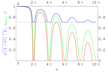
Figure 3: (Color online) Plot of the maximal Bell inequality violation $B_{max}$ (middle green plot) as a function of the deviation from the coincidence of the current measurements: $\alpha=\frac{x_{B}-x_{A}}{v_{F}\tau_{V}}$, for the case of small measurement times: $\tau\ll\hbar/eV$. $B_{max}$ is sandwiched between the plot for concurrence ${\bf C}$ (lower red plot) for orbital part of the two-particle density matrix: $\hat{\rho}_{AB}$, and the plot for the function: $\sqrt{\frac{1+{\bf C}^{2}}{2}}$ (upper blue plot). The doted line at $1/\sqrt{2}$ marks the critical value above which the Bell inequality is violated. The transmission probability is taken to be: $\gamma\approx\epsilon^{2}=0.001$.

A natural question to ask is whether entanglement can occur between orbital and spin degrees of freedom. Starting from the general density matrix of Eq. (20), it is possible to perform a partial trace with respect to a single spin and a single pseudo spin, in order to test this property. We do not show this computation, but instead mention only the result: the concurrence is strictly zero. In any case, if no trace of the density matrix (20) is performed, we conjecture that the joined state of spin and orbital degrees of freedom can be a hyperentangled state PRL_72_052110 . In quantum optics these states can be used for instance to measure the concurrence directly Nature_440_1022 .

V Calculation of current cross-correlations

The theoretical calculation of the concurrence cannot easily be tested experimentally: it would require quantum state tomography, which represents a considerable challenge in experimental mesoscopic physics. A theoretical proposal for tomography has been been presented recently samuelson_tomography , which relies on the measurement of zero frequency noise cross-correlations. Because of the considerable experimental challenge of tomography and because we wish to compare different diagnosis for quantum mechanical non-locality, here we present a Bell violation test based on the analysis of short time current cross-correlations. Here we are interested in the same quantities for the specific setup of Fig. 2, evaluated at points in the leads: $A_{1}$, $A_{2}$, $B_{3}$ and $B_{4}$.

We continue using scattering theory for NS-systems. Our starting point is the current operator in lead $i$:

$$\hat{I}_{i}(x)=\frac{ie\hbar}{2m}\sum_{\sigma}\left[\frac{\partial\Psi_{i,\sigma}^{+}(x)}{\partial x}\Psi_{i,\sigma}(x)-\Psi_{i,\sigma}^{+}(x)\frac{\partial\Psi_{i,\sigma}(x)}{\partial x}\right],$$ (31)

this operator is expressed in terms of electron and hole wave functions:

$$\hat{I}_{i}(x)=\frac{ie\hbar}{2mv_{F}}\frac{1}{2\pi\hbar}\int_{0}^{+\infty}dE_{1}\int_{0}^{+\infty}dE_{2}\sum_{m,n}\sum_{\sigma}$$

$$\;\;\;\;\;\;\;\;\left[(u_{in}\partial_{x}u_{im}^{*}-\partial_{x}u_{in}u_{im}^{*})\hat{c}_{m\sigma}^{+}\hat{c}_{n\sigma}\right.$$

$$\;\;\;\;\;\;\;\;-{\sigma}(v_{in}^{*}\partial_{x}u_{im}^{*}-\partial_{x}v_{in}^{*}u_{im}^{*})\hat{c}_{m\sigma}^{+}\hat{c}_{n-\sigma}^{+}$$

$$\;\;\;\;\;\;\;\;-{\sigma}(u_{in}\partial_{x}v_{im}-\partial_{x}u_{in}v_{im})\hat{c}_{m-\sigma}\hat{c}_{n\sigma}$$

$$\;\;\;\;\;\;\;\;\left.+(v_{in}^{*}\partial_{x}v_{im}-\partial_{x}v_{in}^{*}v_{im})\hat{c}_{m-\sigma}\hat{c}_{n-\sigma}^{+}\right],$$ (32)

where we have replaced the sums over $j$ and $\beta$ by a single sum other index $m$. The terms with index $m$ ($n$) corresponds to energy $E_{1}$ ($E_{2}$). The chemical potential $\mu_{S}$ of the superconductor is large compared to any other energy scale in the system, thus the assumption $k_{e}=k_{h}=k_{F}$ is made here, which explains the presence of the Fermi velocity $v_{F}$ in Eq. (32).

The calculation of current correlations is rather standard, but it is reproduced in the Appendix so that the notations of the present work can be understood. Compared to the calculation of the density matrix of Sec. 3, the characterization of the scattering properties of the setup of Fig. 2 now requires to include the MZ interferometers. The magnetic fluxes which are applied on the left ($\Phi_{A}$) and on the right ($\Phi_{B}$) interferometers define the Bell angles:

$$\varphi_{A}=2\pi\frac{\Phi_{A}}{\Phi_{0}},\;\;\;\;\;\;\;\;\varphi_{B}=2\pi\frac{\Phi_{B}}{\Phi_{0}},$$ (33)

In analogy with spin entanglement of electrons kawabata ; chtchelkatchev , where electrons are detected via spin filters with arbitrary polarization, the phase angles $\varphi_{A}$ and $\varphi_{B}$ allow to rotate the pseudo-spins with respect to the $\hat{Z}$ axis, which is defined in a basis $|\uparrow\rangle=|u\rangle$ and $|\downarrow\rangle=|d\rangle$. Indeed, electron wave functions gain a factor $e^{\pm i\varphi_{A,B}/2}$ in the upper/lower arms of the interferometers, which is equivalent to a rotation by the angle $\varphi_{A,B}$ in the pseudo-spin basis. Next, the use of a symmetric beam splitter, which is described by a unitary matrix,

$$U=\left(\begin{array}[]{ccc}\frac{1}{\sqrt{2}}&\frac{i}{\sqrt{2}}\\ \frac{i}{\sqrt{2}}&\frac{1}{\sqrt{2}}\end{array}\right),$$ (34)

performs a rotation of such pseudo-spin around the $\hat{Y}$-axis by an angle $\pi/2$. In the end, the latter measurements at the points $A_{1}$,$A_{2}$ (left side of Fig. 2) and $B_{3}$,$B_{4}$ (right side of Fig. 2) correspond to a Stern-Gerlach type of measurement along $\hat{Z}$ axis for the initial pseudo-spins. These transformations on both the right and the left orbital pseudo-spins allow to perform standard Bell type correlation measurements.

For constructing the scattering amplitudes, we use $A$, $B$, $C$, $D$ from Eqs. (15a)-(15d) and the elements of the beam splitter scattering matrix Eq. (34). The following convention is used for the angle signs: an electron-like quasiparticle on the left (right) side gains a phase $e^{+i\varphi_{A}/2}$ ($e^{-i\varphi_{B}/2}$), when it propagates in the clockwise direction through the upper arm of the interferometer. For anticlockwise movement the sign in the exponent is opposite. For a hole-like quasiparticle moving clockwise in the lower arm the sign is also opposite.

Note that this convention applies to the case where the direction of the magnetic field is opposite in different interferometers. This situation may seem hard to realize experimentally, however it was chosen only for convenience: in the contrary situation (with both fields in the same direction) one simply needs to change the sign of an angle in (33).

For a given type of particle (electron or hole), the scattering matrices have dimensions of $4\times 4$, which corresponds to the number of leads attached to the superconductor: recall that here we are working in the Andreev regime. In order to write the matrices, we use the amplitudes in Eqs. (15a)-(15d), an angle $\delta\varphi=\varphi_{A}-\varphi_{B}$ and unitary matrices for scattering amplitudes of the beam splitters in Eq. (34):

$$\small S^{\alpha\alpha}(+E)=\left(\begin{array}[]{cccc}\frac{A}{2}+\frac{1}{2}&\frac{iA}{2}-\frac{i}{2}&\frac{B}{2}e^{-i\delta\varphi/2}&\frac{iB}{2}e^{-i\delta\varphi/2}\\ \frac{iA}{2}-\frac{i}{2}&-\frac{A}{2}-\frac{1}{2}&\frac{iB}{2}e^{-i\delta\varphi/2}&-\frac{B}{2}e^{-i\delta\varphi/2}\\ \frac{B}{2}e^{+i\delta\varphi/2}&\frac{iB}{2}e^{+i\delta\varphi/2}&\frac{A}{2}+\frac{1}{2}&\frac{iA}{2}-\frac{i}{2}\\ \frac{iB}{2}e^{+i\delta\varphi/2}&-\frac{B}{2}e^{+i\delta\varphi/2}&\frac{iA}{2}-\frac{i}{2}&-\frac{A}{2}-\frac{1}{2}\end{array}\right),$$ (35a)

for $$\alpha\neq\beta$$:

$$\small S^{\alpha\beta}(+E)=-\left(\begin{array}[]{cccc}\frac{C}{2}&\frac{iC}{2}&\frac{D}{2}e^{-i\delta\varphi/2}&\frac{iD}{2}e^{-i\delta\varphi/2}\\ \frac{iC}{2}&-\frac{C}{2}&\frac{iD}{2}e^{-i\delta\varphi/2}&-\frac{D}{2}e^{-i\delta\varphi/2}\\ \frac{D}{2}e^{i\delta\varphi/2}&\frac{iD}{2}e^{i\delta\varphi/2}&\frac{C}{2}&\frac{iC}{2}\\ \frac{iD}{2}e^{i\delta\varphi/2}&-\frac{D}{2}e^{i\delta\varphi/2}&-\frac{iC}{2}&\frac{C}{2}\end{array}\right).$$ (35b)

In these matrices, the terms $\pm\frac{1}{2}$ and $+\frac{i}{2}$ in the scattering amplitudes originate from the full reflection of a particle approaching an ideal energy filter, as specified by Eqs. (16b)-(16e), which is adjusted not to allow the transmission of a particle with this particular energy. The amplitudes for energies below Fermi level ($-E$) are calculated using the property of Eq. (63).

Note that here we did not include explicitly factors such as $e^{\pm k_{e/h}l}$, which correspond to phases accumulated by particles propagating through a lead of length $l$. These phases can be included as an overall multiplication factor on the scattering matrix in Eqs. (71a)-(71c), depending on the lead coordinate. Here the assumption that both arms of any given MZ interferometer have the same length is implicit. We also neglect the length $S$ of the injecting lead of the superconducting fork, and we assume an ideal NS-boundary in the pure Andreev reflection regime with amplitudes: $r_{SS}^{eh}=r_{SS}^{he}=e^{-i\eta}=-i$.

From the scattering amplitudes of Eqs. (35a)-(35b) we obtain the noise cross-correlations, which may be separated in an excess and an equilibrium parts:

$$C(x_{i},t_{i};x_{j},t_{j})=C_{ex}(x_{i},t_{i};x_{j},t_{j})+C_{eq}(x_{i},t_{i};x_{j},t_{j}),$$

the excess part (first term) depends on voltage and originates from the first term in Eqs. (71a)-(71c), the equilibrium part(second term) is voltage independent and it occurs from the second term (delta functions) in Eqs. (71a)-(71c).

It is then natural to introduce time scales which characterize the time spacing between electron wave packets, as well as the time of flight of particle through the wires: $\tau_{V}=\hbar/eV$, $\tau_{ij}^{eq}=(|x_{j}|+|x_{i}|)/v_{F}$ and $\tau_{ij}^{ex}=(|x_{j}|-|x_{i}|)/v_{F}$. In addition, $\tau_{ij}=t_{j}-t_{i}$. So the cross-correlations at finite temperature $T$ reads:

$$C^{ex}_{ij}(\tau_{ij},\tau_{ij}^{ex},T)=\frac{2e^{2}}{h^{2}}\frac{\epsilon^{2}(1-2\epsilon-\epsilon^{2})}{8(1-\epsilon)^{4}}$$

$$\;\;\;\;\times(1+(-1)^{i+j}\cos{(\delta\varphi-(\tau_{ij}-\tau_{ij}^{ex})/\tau_{V})})$$

$$\;\;\;\;\times 4\sin^{2}\frac{(\tau_{ij}-\tau_{ij}^{ex})}{2\tau_{V}}\frac{(\pi T)^{2}}{\sinh^{2}(\pi T(\tau_{ij}-\tau_{ij}^{ex})/\hbar)},$$ (36)

$$C^{eq}_{ij}(\tau_{ij},\tau_{ij}^{eq},T)=-\frac{2e^{2}}{h^{2}}\frac{1+\sqrt{1-2\epsilon}-(2+\sqrt{1-2\epsilon})\epsilon}{8(1-\epsilon)^{2}}$$

$$\times\left[\frac{(\pi T)^{2}}{\sinh^{2}(\pi T(\tau_{ij}+\tau_{ij}^{eq})/\hbar)}+\frac{(\pi T)^{2}}{\sinh^{2}(\pi T(\tau_{ij}-\tau_{ij}^{eq})/\hbar)}\right].$$

For zero temperature ($k_{B}T\ll eV$), the correlators reduce to:

$$C^{ex}_{ij}(\tau_{ij},\tau_{ij}^{ex},0)=\frac{2e^{4}V^{2}}{h^{2}}\frac{\epsilon^{2}(1-2\epsilon-\epsilon^{2})}{8(1-\epsilon)^{4}}\frac{\sin^{2}\left(\frac{\tau_{ij}-\tau_{ij}^{ex}}{2\tau_{V}}\right)}{\left(\frac{\tau_{ij}-\tau_{ij}^{ex}}{2\tau_{V}}\right)^{2}}$$

$$\;\;\;\;\;\;\;\;\times(1+(-1)^{i+j}\cos{(\delta\varphi-(\tau_{ij}-\tau_{ij}^{ex})/\tau_{V})}),$$ (37)

$$C^{eq}_{ij}(\tau_{ij},\tau_{ij}^{eq},0)=-\frac{2e^{2}}{(2\pi)^{2}}\frac{1+\sqrt{1-2\epsilon}-(2+\sqrt{1-2\epsilon})\epsilon}{8(1-\epsilon)^{2}}$$

$$\;\;\;\;\;\;\;\;\;\;\;\;\;\;\;\;\times\left[\frac{1}{(\tau_{ij}+\tau_{ij}^{eq})^{2}}+\frac{1}{(\tau_{ij}-\tau_{ij}^{eq})^{2}}\right].$$ (38)

Note that the equilibrium noise describes Fermi correlations within the normal leads. At low temperatures it decays as an inverse square with large distances from the superconducting fork to the detectors. So assuming large distances, $x_{i},\;x_{j}\gg v_{F}\tau_{V}$, only excess noise is relevant, and this corresponds to the excess noise due to Cooper pairs injected from the superconductor. The dependence on magnetic fluxes in the excess noise occurs via $\delta\varphi=\varphi_{A}-\varphi_{B}$. One should therefore attempt to construct a Bell type inequality with these measurable quantities.

VI Bell test for current correlations

In optics, the Bell inequality test is typically expressed in terms of correlators of number operators. This reflects the fact that a coincidence measurement on two photons is performed. In Refs. lesovik_martin_blatter and chtchelkatchev , these number correlators were expressed in terms of current noise cross-correlators, which contain an irreducible contribution and a reducible contribution. The reducible contribution is proportional to the product of the average current in each lead. The irreducible contribution dominates for short observation times. Subsequently, the Bell inequality can be written in terms of irreducible zero frequency noise cross-correlators between the different arms of the device. A slightly different point of view was proposed in orbital_entanglement and discussed in Entanglement4 : As long as the spacing in time between electron wave packets $e/\langle I\rangle$ is large compared to the size of these wave packets $\hbar/eV$, successive pairs do not mix so that all information about entanglement is included in the zero frequency noise correlators.

In this letter, we suggest a Bell type inequality for finite time cross-correlations of electrical currents. It is similar in spirit as in work of Ref. Entanglement3, ; Entanglement4, , where Bell inequalities are directly expressed in terms of current correlators, yet we shall see that our analysis is not necessarily restricted to short times. We thus follow the derivation of Ref. chtchelkatchev, for the Bell inequality violation with particle numbers:

$$\left|E(\varphi_{a},\varphi_{b})+E(\varphi_{a},\varphi_{b}^{\prime})+E(\varphi_{a}^{\prime},\varphi_{b})-E(\varphi_{a}^{\prime},\varphi_{b}^{\prime})\right|\leq 2,$$ (39)

where

$$E(\varphi_{a},\varphi_{b})=\frac{\left\langle(N_{1}(\tau)-N_{2}(\tau))(N_{3}(\tau)-N_{4}(\tau))\right\rangle}{\left\langle(N_{1}(\tau)+N_{2}(\tau))(N_{3}(\tau)+N_{4}(\tau))\right\rangle},$$ (40)

and with $\varphi_{a}$, $\varphi_{b}$ - angles corresponding to different magnetic fluxes in the left and the right interferometers. $\tau$ is the duration of the measurement in time. Particle number operators in different leads $A_{1}$-$B_{4}$ are defined from current operators: $N_{i}(t,\tau)=\int_{t}^{t+\tau}dt^{\prime}I_{i}(t^{\prime})$. We perform density matrix averaging and time averaging:

$$\left\langle N_{i}(\tau)N_{j}(\tau)\right\rangle=\lim_{T\rightarrow\infty}\frac{1}{2T}\int_{-T}^{+T}dt\left\langle N_{i}(t,\tau)N_{j}(t,\tau)\right\rangle_{\rho}~{}.$$ (41)

We define the irreducible current cross-correlator at given positions and times $t_{1}$ and $t_{2}$:

$$C_{ij}(t_{2}-t_{1},x_{i},x_{j})=\left\langle\hat{I}_{i}(x_{i},t_{1})\hat{I}_{j}(x_{j},t_{2})\right\rangle$$

$$\;\;\;\;\;\;\;\;\;\;\;\;\;\;\;\;-\left\langle\hat{I}_{i}(x_{i},t_{1})\right\rangle\left\langle\hat{I}_{j}(x_{j},t_{2})\right\rangle,$$ (42)

and we write the Bell term in the following form:

$$\small E(\varphi_{a},\varphi_{b})=\frac{\int_{0}^{\tau}dt_{1}\int_{0}^{\tau}dt_{2}(C_{13}-C_{14}-C_{23}+C_{24})+\Lambda_{-}}{\int_{0}^{\tau}dt_{1}\int_{0}^{\tau}dt_{2}(C_{13}+C_{14}+C_{23}+C_{24})+\Lambda_{+}},$$ (43)

where $\Lambda_{\pm}$ originate from the reducible part, which is typically proportional to the average currents:

$$\Lambda_{\pm}=\tau^{2}\left(\left\langle I_{1}\right\rangle\pm\left\langle I_{2}\right\rangle\right)\left(\left\langle I_{3}\right\rangle\pm\left\langle I_{4}\right\rangle\right).$$ (44)

The coordinates $x_{i}$ and $x_{j}$ in Eq. (42) correspond to positions of the detectors counted from the superconducting fork, and $\tau$ correspond to duration of measurements.

For the case of symmetrical beam splitters used in interferometers and a symmetrical superconducting fork the average electrical currents are identical: $\left\langle I_{i}\right\rangle=\frac{e^{2}V}{h}\frac{\epsilon^{2}}{(1-\epsilon)^{2}}$, so $\Lambda_{-}=0$ and

$$\small\Lambda_{+}=4\tau^{2}\frac{e^{2}V}{h}\frac{\epsilon^{2}}{(1-\epsilon)^{2}}.$$ (45)

In this case the Bell term reads:

$$\small E(\varphi_{a},\varphi_{b})=\frac{\int_{0}^{\beta}dt_{1}\int_{0}^{\beta}dt_{2}\frac{\sin^{2}\frac{t_{2}-t_{1}+\alpha}{2}}{(t_{2}-t_{1}+\alpha)^{2}}\cos{\left(\delta\varphi-(t_{2}-t_{1}+\alpha)\right)}}{\int_{0}^{\beta}dt_{1}\int_{0}^{\beta}dt_{2}\frac{\sin^{2}\frac{t_{2}-t_{1}+\alpha}{2}}{(t_{2}-t_{1}+\alpha)^{2}}+\gamma\beta^{2}},$$ (46)

here $\alpha=\frac{x_{B}-x_{A}}{v_{F}\tau_{V}}$. For simplicity, we consider the case where $x_{1}=x_{2}=x_{A}$ and $x_{3}=x_{4}=x_{B}$, assuming a precision $\delta x\ll v_{F}\tau_{V}$ - i.e. the detectors of each party $A$ and $B$ are equidistant from the superconducting fork. Moreover, $\beta=\tau/\tau_{V}$, $\gamma=\frac{\epsilon^{2}}{1-2\epsilon-\epsilon^{2}}$, $\delta\varphi=\varphi_{a}-\varphi_{b}$. So there are three dimensionless parameters: $\alpha$ - which describes the fact that the measurements performed by $A$ and $B$ parties are not in coincidence; $\beta$ - the duration of these measurements, $\gamma$ - the parameter describing the transport properties of the superconducting fork (recall that it depends only on $\epsilon$, which is the probability of a particle to go from the injection lead into one of the two leads); and $\delta\varphi$ is the difference between the Bell angles introduced in Eq. (33).

In our analysis of the Bell inequality of Eq. (39) we consider two simple cases, for both of them the Bell term in Eq. (40) satisfies $E(\varphi_{a},\varphi_{b})\sim\cos{(\varphi_{a}-\varphi_{b})}$.

i) The case of coincident measurements: $\alpha=0$. On Fig. 4 we show the resulting dependence of the maximal Bell inequality violation $B_{max}$ (which is the maximum of the left side of the Bell inequality over the Bell angles) over the measurement time $\tau$. From Fig. 4 it is clear, that for the case of superconducting fork with very bad transmission ($\epsilon\to 0$, $\gamma\to 0$), the violation of Bell inequality is possible only for $\tau<2\tau_{V}$. We again stress that long measurement times destroy the interference between trajectories with different energies, so that the Bell inequality cannot be violated.

In our analysis, the maximal violation depends on the transmission properties of the superconducting fork: the closer $\gamma$ to zero the better the violation. The Bell inequality in Eq. (39) may be violated maximally (with $\beta\to 0$) for $\epsilon\to 0$, and it is not violated at all for $\epsilon\geq\epsilon_{max}=(3-\sqrt{2})/7\approx 0.22$ [this corresponds to: $\gamma\geq\gamma_{max}=(\sqrt{2}-1)/4$]. This fact may by explained in the following way: the irreducible cross-correlations vanishes when $\gamma\to\pm\infty$ (See Ref. Noise3, ). Indeed, the term of Eq. (37) equals to zero for $\epsilon_{0}=\sqrt{2}-1\approx 0.42$.

Figure 4: Plot for the maximal Bell inequality violation $B_{max}$ as a function of the measurement time: $\beta=\tau/\tau_{V}$. The analysis is performed in terms of current cross-correlations, the deviation from the coincidence of measurement times $\alpha=\frac{x_{B}-x_{A}}{v_{F}\tau_{V}}$ is taken to be zero. The maximally possible violation is normalized to $1$, thus the limit for Bell inequality violation is $1/\sqrt{2}$. The transmission probability $\epsilon$ is the same as in Fig. 3.

ii) The case of short time measurements: $\beta\rightarrow 0$. Here we vary two parameters: $\epsilon$ - the transparency of the superconducting fork, which defines the parameter $\gamma=\frac{\epsilon^{2}}{1-2\epsilon-\epsilon^{2}}$, and $\alpha=\frac{x_{B}-x_{A}}{v_{F}\tau_{V}}$ - which characterizes the lack of coincidence of the measurements by the two parties $A$ and $B$. Again, the best violation occurs for $\alpha\to 0$, and there is a dependence of maximal violation on transmission properties of the fork, which are described by $\gamma$. The Bell inequality in this case is the following:

$$B_{max}=\left|\frac{\sin^{2}{\frac{\alpha}{2}}}{\sin^{2}{\frac{\alpha}{2}}+\gamma\alpha^{2}}\right|\leq\frac{1}{\sqrt{2}},$$ (47)

where we have chosen the Bell angles: $\delta\varphi_{ab}=\delta\varphi_{ab^{\prime}}=\delta\varphi_{a^{\prime}b}=\pi/4-\alpha$, $\delta\varphi_{a^{\prime}b^{\prime}}=3\pi/4-\alpha$, for which the violation is maximal. The dependence of these angles on $\alpha$ is due to the presence of $\alpha$ under the cosine in Eq. (46).

In Fig. 3 we plot the dependence of the left hand side of the Bell inequality on $\alpha$, for a certain $\gamma=0.001$. There is again a threshold in the transparency $\epsilon_{max}=0.22$, below which the violation is possible. For a transmission probability below the threshold $\epsilon_{max}$ the Bell inequality in Eq. (47) can be violated for: $\alpha\leq\tau_{V}\sqrt{(\sqrt{2}-1)/\gamma}\approx 0.6\tau_{V}/\epsilon$, while it remains inviolated in narrow regions separated by intervals: $\frac{h}{eV}$.

To compare the entanglement measure and the maximal Bell inequality violation, we plot in the same Fig. 3 the concurrency ${\bf C}$ as well as the function $\sqrt{\frac{1+{\bf C}^{2}}{2}}$. It is known gisin that for mixed states $B_{max}$ is confined between these two values (for the case of pure states $B_{max}\equiv\sqrt{\frac{1+{\bf C}^{2}}{2}}$), which is clearly seen from the plots of Fig. 3. According to our results, there may occur situations, where the state on the detectors is entangled (${\bf C}\neq 0$), but there is no Bell inequality violation ($B_{max}<1/\sqrt{2}$).

From these two examples of i) $\alpha=0$ and ii) $\beta=0$ we conclude that the violation of Bell inequality occurs for small measurement times: $\tau<2\tau_{V}$ and for measurements which are close to being coincident: $|x_{A}-x_{B}|/v_{F}<0.6\tau_{V}/\epsilon$. We performed numerical integrations of Eq. (46) for arbitrary values of $\{\alpha,\beta,\gamma\}$. The results for $\gamma=0.001$ and $\gamma=\gamma_{max}\approx 0.1$ are shown on two-dimensional plots of Fig. 5 and of Fig. 6. Note that the plot of Fig. 3 represent a slice at $\alpha=0$ of Fig. 5, while Fig. 4 represents a slice at $\beta=0$ of the same figure. One notices that the oscillations of $B_{max}$ are damped as $\alpha$ is increased, and, as mentioned above that violation is less likely when $\beta$ is increased because the time window is too large. Such oscillations in the Bell parameter were detected previously in the case of normal metal forks Entanglement4 . It is obvious from Fig. 6 that, when the transparency of the superconducting fork is larger than the critical threshold, there is no violation of the Bell inequalities, although oscillations are still noticeable.

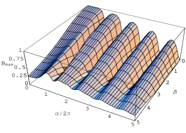
Figure 5: (Color online) Plot for the maximal Bell inequality violation $B_{max}$ depending both on the deviation from coincidence of current measurements: $\alpha=\frac{x_{B}-x_{A}}{v_{F}\tau_{V}}$ and the measurement time $\beta\tau\ll\hbar/eV$. The maximal value is normalized to unity. The transmission probability is taken to be: $\gamma\approx\epsilon^{2}=0.001$. Violation above the critical value of $1/\sqrt{2}$ occurs only at separate peak locations.

VII Conclusion.

We have proposed a setup measuring energy entanglement for pairs of quasiparticles originating from single Cooper pairs in a superconductor. The use of energy filters allows to separate the particles according to their energy and to obtain orbitally entangled pairs of electrons, which are then analyzed. This electronic setup and its detection apparatus is an analog of the momentum-phase entanglement performed in quantum optics rarity . a) Two electrons from a Cooper pair correspond to the two photons generated by down-conversion, which have different wave lengths. Indeed, Andreev reflection, or the emission of a Cooper pair, also involves two electrons with different energies. b) In optics the spatial separation of the photon beams follows automatically from the down conversion process. Here, we used energy filters to perform such separation and considered short time measurements to allow interference of particles with slightly different energies. It is because the interference occurs between different energies that the “usual” zero-frequency analysis is not applicable here. This is why we developed a Bell inequality test for finite-times cross-correlations of electrical currents.

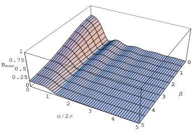
Figure 6: (Color online) Same as Fig. 5, except that the transmission probability is taken to be critical: $\gamma=\gamma_{max}\approx 0.1$. The whole surface lies below the critical value $1/\sqrt{2}$, so there is no violation of the Bell inequality.

First, we proposed a density matrix analysis for quasiparticles emitted from a superconductor and separated in energy. This allows to calculate the concurrence, one of the most widely used entanglement measures. Second, we showed how energy entanglement can be transformed into orbital entanglement and how it then can be tested via electrical current cross-correlations. For such cross-correlations, we constructed a Bell type inequality and showed what set of parameters lead to its violation.

The noise cross-correlations between the left and the right reservoirs were derived in the context of the scattering theory for normal metal-superconductor hybrid circuits. Indeed, in stationary quantum transport these correlations enter explicitly the Bell inequality test. Here the manifestation of entanglement is found by adjusting the phases accumulated by electrons and holes in the conductor leading to the beam splitter (one can change magnetic fluxes within MZ interferometers by varying the magnetic field through them or by varying their area, like it was done in experiments with a single interferometer MZ_for_electrons ). For a device consisting of perfect elements (filters, beam splitters,…), maximal Bell violation is obtained for short time of measurements: $\tau<2\tau_{V}$ and small deviations from coincident measurements between the left and the right reservoirs: $|x_{A}-x_{B}|/v_{F}<0.6\tau_{V}/\epsilon$ - for relatively small transparency $\epsilon$ of the superconducting fork. We found that the violation of the Bell inequality depends on transmission properties of the fork, and it occurs for: $\epsilon<\epsilon_{max}\approx 0.22$.

A clear issue is to inquire whether such energy entanglement can be detected in experiments. Our setup for generating entangled electron pairs has many components, each of which in principle can be built for instance using gated semiconductor hetero-structures. The design of a controllable normal metal-superconducting fork represents a challenge but, recently, work in this direction has been promising schonenberger . All leads are assumed one dimensional, and are assumed to have little or no backscattering as, for instance, in the experiments of Ref. auslaender . The energy filtering fork can be constructed from an ordinary fork with coherent quantum dots at two ends of it. The dots are adjusted to have transmission peaks symmetrically above and below the Fermi level. For better filtering these dots must have levels with an energy spacing larger than the bias voltage.

Because of the complexity of this device, there are other complications which should be considered. The setup is composed of two MZ interferometers, which are both subject to dephasing marquard . The fluctuations in the gate voltages could trigger fluctuations in the path length, which consequently would add an uncertainty to the phase of electrons and holes, which enter the noise correlation expression of Eq. (37). As long as the phase fluctuations are controlled (small compared to a phase angle $\pi$, meaning that the fluctuations in path length are below the Fermi wave length $\lambda_{F}$), the Bell inequality will continue to be violated. Furthermore, a considerable precision is required in the building of such an interferometer: the two arms need to have equal length, up to a distance $v_{F}\tau_{V}>\lambda_{F}$.

In conclusion, we have proposed the first energy entanglement setup for testing the non-locality properties of electrons in nanostructures. With the previous work on spin entanglement using NS junctions, this latest work emphasizes the analogy with quantum optics. Our main goal here has been to show that energy entanglement can in principle be analyzed (concurrence) or detected (noise cross-correlation analysis) in this somewhat ideal device, using concepts and circuitry borrowed from mesoscopic physics.

We thank Andrey Lebedev and Pavel Ostrovsky for fruitful discussions and helpful comments. K.B. acknowledges support by the ENS-Landau exchange program. G.L. and K.B. acknowledges support from the Russian Foundation for Basic Research, grant 06-02-17086-a. T.M. acknowledges support from an AC Nanosciences and from the ACI Jeunes Chercheurs (Lefloch) funding programs of CNRS.

Appendix A Density matrix

Starting from Eqs. (5)-(11) we average two anihilation operators products as:

$$\left\langle\hat{c}_{m\sigma}^{+}(E_{1})\hat{c}_{n\sigma}(E_{2})\right\rangle=f_{m}\delta_{mn}\delta(E_{1}-E_{2})~{},$$ (48)

where $f_{m}=f_{FD}(E{\mp}eV)$ for electrons and holes, with $f_{FD}(E)$ the Fermi-Dirac distribution. And averages of four operators are calculated using Wick’s theorem:

$$\;\;\;\;\;\;\;\;\;\;\;\;\;\;\;\;\left\langle\hat{c}_{k\sigma_{1}^{\prime}}^{\dagger}(E_{1},t_{i^{\prime}})\hat{c}_{l\sigma_{2}^{\prime}}^{\dagger}(E_{2},t_{j^{\prime}})\hat{c}_{m\sigma_{2}}(E_{3},t_{j})\hat{c}_{n\sigma_{1}}(E_{4},t_{i})\right\rangle=$$

$$=f_{k}(E_{1})f_{l}(E_{2})\delta_{\sigma_{1}^{\prime}\sigma_{1}}\delta_{\sigma_{2}^{\prime}\sigma_{2}}\delta_{kn}\delta_{lm}\delta(E_{1}-E_{4})\delta(E_{2}-E_{3})e^{-iE_{1}(t_{i}-t_{i^{\prime}})/\hbar}e^{+iE_{2}(t_{j}-t_{j^{\prime}})/\hbar}$$

$$-f_{k}(E_{1})f_{l}(E_{2})\delta_{\sigma_{1}^{\prime}\sigma_{2}}\delta_{\sigma_{2}^{\prime}\sigma_{1}}\delta_{km}\delta_{ln}\delta(E_{1}-E_{3})\delta(E_{2}-E_{4})e^{-iE_{1}(t_{j}-t_{i^{\prime}})/\hbar}e^{+iE_{2}(t_{j^{\prime}}-t_{i})/\hbar}.$$ (49)

The resulting calculation leads to appearance of three terms with different spin symmetry:

$$\;\;\;\;\;\;\;\;g(\vec{\sigma},\vec{x})=\frac{1}{(hv_{F})^{2}}\sum\limits_{k,l}\int_{0}^{+\infty}\int_{0}^{+\infty}dE_{1}dE_{4}$$ (50)

$$\left\{\delta_{\sigma_{1}\sigma_{1}^{\prime}}\delta_{\sigma_{2}\sigma_{2}^{\prime}}\left[(u_{i^{\prime}k}^{*}(x_{i^{\prime}})u_{ik}(x_{i}))(u_{jl}(x_{j})u_{j^{\prime}l}^{*}(x_{j^{\prime}}))e^{-iE_{1}(t_{i}-t_{i^{\prime}})}e^{+iE_{2}(t_{j^{\prime}}-t_{j})}f_{k}(E_{1})f_{l}(E_{2})\right.\right.$$ (51)

$$\;\;\;\;\;\;\;\;\;\;\;\;\;\;\;\;\;+(u_{i^{\prime}k}^{*}(x_{i^{\prime}})u_{ik}(x_{i}))(v_{jl}^{*}(x_{j})v_{j^{\prime}l}(x_{j^{\prime}}))e^{-iE_{1}(t_{i}-t_{i^{\prime}})}e^{-iE_{2}(t_{j^{\prime}}-t_{j})}f_{k}(E_{1})(1-f_{l}(E_{2}))$$ (52)

$$\;\;\;\;\;\;\;\;\;\;\;\;\;\;\;\;\;+(v_{i^{\prime}k}(x_{i^{\prime}})v_{ik}^{*}(x_{i}))(u_{jl}(x_{j})u_{j^{\prime}l}^{*}(x_{j^{\prime}}))e^{+iE_{1}(t_{i}-t_{i^{\prime}})}e^{+iE_{2}(t_{j^{\prime}}-t_{j})}(1-f_{k}(E_{1}))f_{l}(E_{2})$$ (53)

$$\left.\;\;\;\;\;\;\;\;\;\;\;\;\;\;\;\;\;+(v_{i^{\prime}k}(x_{i^{\prime}})v_{ik}^{*}(x_{i}))(v_{jl}^{*}(x_{j})v_{j^{\prime}l}(x_{j^{\prime}}))e^{+iE_{1}(t_{i}-t_{i^{\prime}})}e^{-iE_{2}(t_{j^{\prime}}-t_{j})}(1-f_{k}(E_{1}))(1-f_{l}(E_{2}))\right]$$ (54)

$$-\delta_{\sigma_{1}\sigma_{2}^{\prime}}\delta_{\sigma_{2}\sigma_{1}^{\prime}}\left[(u_{i^{\prime}k}^{*}(x_{i^{\prime}})u_{jk}(x_{j}))(u_{il}(x_{i})u_{j^{\prime}l}^{*}(x_{j^{\prime}}))e^{-iE_{1}(t_{j}-t_{i^{\prime}})}e^{+iE_{2}(t_{j^{\prime}}-t_{i})}f_{k}(E_{1})f_{l}(E_{2})\right.$$ (55)

$$\;\;\;\;\;\;\;\;\;\;\;\;\;\;\;\;\;+(u_{i^{\prime}k}^{*}(x_{i^{\prime}})u_{jk}(x_{j}))(v_{il}^{*}(x_{i})v_{j^{\prime}l}(x_{j^{\prime}}))e^{-iE_{1}(t_{j}-t_{i^{\prime}})}e^{-iE_{2}(t_{j^{\prime}}-t_{i})}(1-f_{l}(E_{2}))$$ (56)

$$\;\;\;\;\;\;\;\;\;\;\;\;\;\;\;\;\;+(v_{i^{\prime}k}(x_{i^{\prime}})v_{jk}^{*}(x_{j}))(u_{il}(x_{i})u_{j^{\prime}l}^{*}(x_{j^{\prime}}))e^{+iE_{1}(t_{j}-t_{i^{\prime}})}e^{+iE_{2}(t_{j^{\prime}}-t_{i})}(1-f_{k}(E_{1}))f_{l}(E_{2})$$ (57)

$$\left.\;\;\;\;\;\;\;\;\;\;\;\;\;\;\;\;\;+(v_{i^{\prime}k}(x_{i^{\prime}})v_{jk}^{*}(x_{j}))(v_{il}^{*}(x_{i})v_{j^{\prime}l}(x_{j^{\prime}}))e^{+iE_{1}(t_{j}-t_{i^{\prime}})}e^{-iE_{2}(t_{j^{\prime}}-t_{i})}(1-f_{k}(E_{1}))(1-f_{l}(E_{2}))\right]$$ (58)

$$+I_{\sigma_{1}\sigma_{2}}I_{\sigma_{1}^{\prime}\sigma_{2}^{\prime}}\left[(u_{i^{\prime}k}^{*}(x_{i^{\prime}})v_{j^{\prime}k}(x_{j^{\prime}}))(u_{il}(x_{i})v_{jl}^{*}(x_{j}))e^{-iE_{1}(t_{j^{\prime}}-t_{i^{\prime}})}e^{+iE_{2}(t_{j}-t_{i})}f_{k}(E_{1})f_{l}(E_{2})\right.$$ (59)

$$\;\;\;\;\;\;\;\;\;\;\;\;\;\;\;\;\;-(u_{i^{\prime}k}^{*}(x_{i^{\prime}})v_{j^{\prime}k}(x_{j^{\prime}}))(v_{il}^{*}(x_{i})u_{jl}(x_{j}))e^{-iE_{1}(t_{j^{\prime}}-t_{i^{\prime}})}e^{-iE_{2}(t_{j}-t_{i})}f_{k}(E_{1})(1-f_{l}(E_{2}))$$ (60)

$$\;\;\;\;\;\;\;\;\;\;\;\;\;\;\;\;\;-(v_{i^{\prime}k}(x_{i^{\prime}})u_{j^{\prime}k}^{*}(x_{j^{\prime}}))(u_{il}(x_{i})v_{jl}^{*}(x_{j}))e^{+iE_{1}(t_{j^{\prime}}-t_{i^{\prime}})}e^{+iE_{2}(t_{j}-t_{i})}(1-f_{k}(E_{1}))f_{l}(E_{2})$$ (61)

$$\left.\left.\;\;\;\;\;\;\;\;\;\;\;\;\;\;\;\;\;+(v_{i^{\prime}k}(x_{i^{\prime}})u_{j^{\prime}k}^{*}(x_{j^{\prime}}))(v_{il}^{*}(x_{i})u_{jl}(x_{j}))e^{+iE_{1}(t_{j^{\prime}}-t_{i^{\prime}})}e^{-iE_{2}(t_{j}-t_{i})}(1-f_{k}(E_{1}))(1-f_{l}(E_{2}))\right]\right\},$$ (62)

where we have used the matix notation ($\sigma_{i}=\pm 1$): $I_{\sigma_{1}\sigma_{2}}=i\hat{\tau}_{y}$ and $\hat{\tau}_{y}$ is a Pauli matrix.

We consider the Andreev reflection at the NS-boundary to be ideal (no normal reflection), and the reflection amplitude reads: $r_{A}=e^{-i\arccos{\frac{E}{\Delta}}}$. According to the properties of Bogolubov’s equations the scattering amplitudes must satisfy the equations:

$$S_{ij}^{hh}(E)=S_{ij}^{ee*}(-E),\;\;\;\;S_{ij}^{he}(E)=-S_{ij}^{eh*}(-E),$$ (63)

from this, one can derive the property:

$$v_{ij\beta}(x,E)=(-1)^{\delta_{e\beta}}u_{ij\overline{\beta}}^{*}(x,-E),\;\;\;\;u_{ij\beta}(x,E)=(-1)^{\delta_{h\beta}}v_{ij\overline{\beta}}^{*}(x,-E),$$ (64)

and using the identity $f_{h}(E)=1-f_{e}(-E)$ one can simplify Eqs. (50)-(62):

$$g(\vec{\sigma},\vec{x})=\delta_{\sigma_{1}\sigma_{1}^{\prime}}\delta_{\sigma_{2}\sigma_{2}^{\prime}}G_{i^{\prime}i}G_{jj^{\prime}}^{*}-\delta_{\sigma_{1}\sigma_{2}^{\prime}}\delta_{\sigma_{2}\sigma_{1}^{\prime}}G_{i^{\prime}j}G_{ij^{\prime}}^{*}+I_{\sigma_{1}\sigma_{2}}I_{\sigma_{1}^{\prime}\sigma_{2}^{\prime}}F_{i^{\prime}j^{\prime}}F_{ij}^{*},$$ (65)

where

$$G_{ij}(x_{i},x_{j},t_{j}-t_{i})=\frac{1}{hv_{F}}\sum\limits_{k}\int_{-\infty}^{+\infty}dEf_{k}(E)(u_{ik}^{*}(x_{i})u_{jk}(x_{j}))e^{-iE(t_{j}-t_{i})},$$ (66a)

$$F_{ij}(x_{i},x_{j},t_{j}-t_{i})=\frac{1}{hv_{F}}\sum\limits_{k}\int_{-\infty}^{+\infty}dEf_{k}(E)(u_{ik}^{*}(x_{i})v_{jk}(x_{j}))e^{-iE(t_{j}-t_{i})}.$$ (66b)

Appendix B Current cross-correlations

It is convenient to define the following matrix elements:

$$A_{imin}(E,E^{\prime},x)=u_{in}(E^{\prime},x)\partial_{x}u_{im}^{*}(E,x)-\partial_{x}u_{in}(E^{\prime},x)u_{im}^{*}(E,x),$$ (67a)

$$B_{imin}(E,E^{\prime},x)=v_{in}^{*}(E^{\prime},x)\partial_{x}v_{im}(E,x)-\partial_{x}v_{in}^{*}(E^{\prime},x)v_{im}(E,t),$$ (67b)

$$C_{imin}(E,E^{\prime},x)=u_{in}(E^{\prime},x)\partial_{x}v_{im}(E,x)-\partial_{x}u_{in}(E^{\prime},x)v_{im}(E,x).$$ (67c)

These matrix elements have a useful symmetry:

$$A_{imin}(E,E^{\prime},x)=-A_{inim}^{*}(E^{\prime},E,x),$$ (68a)

$$B_{imin}(E,E^{\prime},x)=-B_{inim}^{*}(E^{\prime},E,x).$$ (68b)

The answer for an average current is the following:

$$\left\langle\hat{I}_{i}(x,t)\right\rangle=\frac{ie}{2\pi mv_{F}}\int_{0}^{+\infty}dE\sum_{m}\left[A_{imim}(E,E,x)f_{m}+B_{imim}(E,E,x)(1-f_{m})\right].$$ (69)

The calculation of irreducible cross-correlation gives:

$$\left\langle\hat{I}_{i}(x_{i},t_{i})\hat{I}_{j}(x_{j},t_{j})\right\rangle-\left\langle\hat{I}_{i}(x_{i},t_{i})\right\rangle\left\langle\hat{I}_{j}(x_{j},t_{j})\right\rangle=\frac{e^{2}\hbar^{2}}{2m^{2}v_{F}^{2}}\frac{1}{(2\pi\hbar)^{2}}\int_{0}^{+\infty}dE\int_{0}^{+\infty}dE^{\prime}\sum_{m,n}$$ (70)

$$\left[f_{m}(E)(1-f_{n}(E^{\prime}))e^{-i(E-E^{\prime})(t_{j}-t_{i})/\hbar}\left[A_{imin}(E,E^{\prime},x_{i})+B_{imin}^{*}(E,E^{\prime},x_{i})\right]\left[A_{jmjn}^{*}(E,E^{\prime},x_{j})+B_{jmjn}(E,E^{\prime},x_{j})\right]\right.$$

$$+f_{m}(E)f_{n}(E^{\prime})e^{-i(E+E^{\prime})(t_{j}-t_{i})/\hbar}C_{inim}^{*}(E^{\prime},E,x_{i})\left[C_{jnjm}(E^{\prime},E,x_{j})+C_{jmjn}(E,E^{\prime},x_{j})\right]$$

$$\left.+(1-f_{m}(E))(1-f_{n}(E^{\prime}))e^{+i(E+E^{\prime})(t_{j}-t_{i})/\hbar}C_{imin}(E,E^{\prime},x_{i})\left[C_{jmjn}^{*}(E,E^{\prime},x_{j})+C_{jnjm}^{*}(E^{\prime},E,x_{j})\right]\right].$$

The averages of products for two and four anihilation operators were calculated using Wick’s theorem in Eq. (49).

In Eq. (70) all terms like in Eqs. (67a)-(67a) may be written in terms of the scattering matrix elements $s_{ij}^{\alpha\beta}$:

$$A_{ik\alpha,il\beta}(E,E^{\prime},x) =2ik_{F}s_{ik}^{e\alpha*}(E)s_{il}^{e\beta}(E^{\prime})e^{+i(E-E^{\prime})\frac{x}{v_{F}\hbar}}-2ik_{F}\delta_{\alpha e}\delta_{\beta e}\delta_{ik}\delta_{il}e^{-i(E-E^{\prime})\frac{x}{v_{F}\hbar}}$$ (71a)

$$B_{ik\alpha,il\beta}(E,E^{\prime},x) =2ik_{F}s_{ik}^{h\alpha}(E)s_{il}^{h\beta*}(E^{\prime})e^{-i(E-E^{\prime})\frac{x}{v_{F}\hbar}}-2ik_{F}\delta_{\alpha h}\delta_{\beta h}\delta_{ik}\delta_{il}e^{+i(E-E^{\prime})\frac{x}{v_{F}\hbar}}$$ (71b)

$$C_{ik\alpha,il\beta}(E,E^{\prime},x) =2ik_{F}s_{ik}^{h\alpha}(E)s_{il}^{e\beta}(E^{\prime})e^{-i(E+E^{\prime})\frac{x}{v_{F}\hbar}}-2ik_{F}\delta_{\alpha h}\delta_{\beta e}\delta_{ik}\delta_{il}e^{+i(E+E^{\prime})\frac{x}{v_{F}\hbar}},$$ (71c)

here we have linearized the $k$-vectors in energy, thus we are not interested in the quadratic behavior of the spectrum near Fermi level and hence we neglect the dispersion of electron and hole wave packets.

References

- (1) D. Bouwmeester, A. Ekert, and A. Zeilinger, The Physics of Quantum Information (Springer-Verlag, Berlin, 2000).
- (2) G. Lesovik, Th. Martin, and G. Blatter, Eur. Phys. J. B 24, 287 (2001).
- (3) P. Recher, E. V. Sukhorukov, and D. Loss, Phys. Rev. B 63, 165314 (2001).
- (4) J. Torrès and T. Martin, Euro. Phys. J. B 12, 319 (1999).
- (5) N.M. Chtchelkatchev, G. Blatter, G.B. Lesovik, and Th. Martin, Phys. Rev. B 66, 161320(R) (2002).
- (6) G. Burkard, D. Loss, and E. V. Sukhorukov, Phys. Rev. B 61, R16303 (2000); G. Burkard and D. Loss, Phys. Rev. Lett. 91, 087903 (2003).
- (7) W. D. Oliver, F. Yamaguchi, and Y. Yamamoto, Phys. Rev. Lett. 88, 037901 (2002); D. S. Saraga, D. Loss, Phys. Rev. Lett. 90, 166803 (2003).
- (8) O. Sauret, T. Martin, D. Feinberg, Phys. Rev. B 72, 024544 (2005).
- (9) Sh. Kawabata, J. Phys. Soc. Jpn., 70, 1210 (2001).
- (10) P. Samuelsson, E. V. Sukhorukov, and M. Büttiker, Phys. Rev. Lett 91, 157002 (2003).
- (11) A.V. Lebedev, G. Blatter, C.W.J. Beenakker, and G.B. Lesovik, Phys. Rev. B 69, 235312 (2004).
- (12) A. V. Lebedev, G. B. Lesovik, G. Blatter, Phys. Rev. B 71, 045306 (2005).
- (13) C. W. J. Beenakker, C. Emary, M. Kindermann, and J. L. van Velsen, Phys. Rev. Lett 91, 147901 (2003).
- (14) P. Samuelsson, E.V. Sukhorukov, M. Büttiker Phys. Rev. Lett. 92, 026805 (2004).
- (15) J.G. Rarity and P.R. Tapster, Phys. Rev. Lett. 64, 2495 (1990).
- (16) D. Boschi, S. Branca, F. De Martini, L. Hardy, and S. Popescu, Phys. Rev. Lett. 80, 1121 (1998).
- (17) C. Simon and Jian-Wei Pan, Phys. Rev. Lett. 89, 257901 (2002).
- (18) S. P. Walborn, S. Padua, and C. H. Monken, Phys. Rev. A 68, 042313 (2003).
- (19) R. Schuster, E. Buks, M. Heiblum, D. Mahalu, V. Umansky, and Hadas Shtrikman, Nature 385, 417 (1997).
- (20) G.B. Lesovik, JETP Lett. 49, 592 (1989).
- (21) M. Büttiker, Phys. Rev. Lett. 65, 2901 (1990).
- (22) M. P. Anantram, S. Datta, Phys. Rev. B 53, 16390 (1996).
- (23) Ya. Blanter, M. Büttiker, Phys. Rep. 336, 1 (2000).
- (24) T. Martin, in Nanoscopic Quantum Transport, (Les Houches session LXXXI, Elsevier 2005), also in arXive:cond-mat/0501208.
- (25) J. Torrès, T. Martin, and G.B. Lesovik, Phys. Rev. B 63, 134517 (2001).
- (26) N.N. Bogolubov, V.V. Tolmachev, and D.V. Shirkov, A New Method in the Theory o Superconductivity, (Consultant Bureau, New York, 1959); P.G. de Gennes, Superconductivity o Metals and Alloys, (Addison Wesley, 1966, 1989).
- (27) B. Shapiro, Phys. Rev. Lett. 50, 747 (1983); Y. Gefen, Y. Imry and M. Ya. Azbel, Phys. Rev. Lett. 52, 129 (1984); M. Büttiker, Y. Imry, and M. Ya. Azbel, Phys. Rev. A, 30, 1982 (1984).
- (28) S. Hill and W.K. Wootters, Phys. Rev. Lett. 78, 5022 (1997); W.K. Wootters, Phys. Rev. Lett. 80, 2245 (1998).
- (29) S. Oh and J. Kim, Phys. Rev. B 71, 144523 (2005).
- (30) V. Coffman, J. Kundu, and W. K. Wootters, Phys. Rev. A 61, 052306 (2000).
- (31) M. Barbieri, C. Cinelli, P. Mataloni, and F. De Martini, Phys. Rev. A 72, 052110 (2005).
- (32) S.P. Walborn, P.H. Souto Ribeiro, L. Davidovich, F. Mintert, and A. Buchleitner, Nature 440, 1002 (2006).
- (33) P. Samuelsson and M. Büttiker, Phys. Rev. B 73, 041305(R) (2006).
- (34) N. Gisin, Phys. Lett. A 154, 201 (1991).
- (35) Y. Ji, Y. Chung, D. Sprinzak, M. Heiblum, D. Mahalu, and H. Shtrikman, Nature 422, 415 (2003).
- (36) B.-R. Choi, A.E. Hansen, T. Kontos, C. Hoffmann, S. Oberholzer, W. Belzig, C. Schonenberger, T. Akazaki, and H. Takayanagi Phys. Rev. B 72, 024501 (2005).
- (37) O. M. Auslaender, A. Yacoby, R. de Picciotto, K. W. Baldwin, L.N. Pfeiffer, and K.W. West, Phys. Rev. Lett. 84, 1764 (2000).
- (38) F. Marquardt and C. Bruder, Phys. Rev. Lett. 92, 056805 (2004).