Phases of Mott-Hubbard bilayers

Abstract

A phase diagram of two Mott-Hubbard planes interacting with a short-range Coulomb repulsion is presented. Considering the case of equal amount of doping by holes in one layer as electrons in the other, a holon-doublon inter-layer exciton formation is shown to be a natural consequence of Coulomb attraction. Quasiparticle spectrum is gapped and incoherent below a critical doping $\delta_{c}$ due to the formation of excitons. A spin liquid insulator (SLI) phase is thus realized without the lattice frustration. The critical value $\delta_{c}$ sensitively depends on the inter-layer interaction strength. In the $tJ$ model description of each layer with the $d$-wave pairing, $\delta_{c}$ marks the crossover between SLI and $d$-wave superconductor. The SLI phase, despite being non-superconducting and charge-gapped, still shows electromagnetic response similar to that of a superfluid due to the exciton transport. Including antiferromagnetic order in the $tJ$ model introduces magnetically ordered phases at low doping and pushes the spin liquid phase to a larger inter-layer interaction strength and higher doping concentrations.

I Introduction

A realization of atomically sharp interface of a band insulator (SrTiO₃) and a Mott insulator (LaTiO₃) and the observation of a metallic interfacial layer between themhwang has prompted a lot of theoretical work on the interfacial phenomena when two insulating materials of completely different physical origin are joined togethermillis ; others . In light of rapid experimental advances in the growth of digitally sharp layered materials, it seems likely that the successful construction of atomically sharp interface between two (doped) Mott insulators is not very far. In fact, a successful construction of alternating LCO:LSCO atomic layers was demonstrated recentlybozovic . A well-known fact that some high-$T_{c}$ materials contain bilayers of doped Hubbard planes adds to the practical importance of studying the bilayer Mott system theoretically. In these regards, a simple yet reliable calculation scheme for understanding the behavior of heterostructure consisting of Mott-insulating materials is called for. We provide one such theoretical framework in this paper. A closely related work considering a correlated bilayer model can be found in Ref. berkeley, .

The situation we have in mind is that of two lightly-doped conducting planes subject to Hubbard-$U$ repulsion, coupled to each other through short-range Coulomb interaction. Each plane is modeled as the Hubbard model, or its large-$U$ equivalent as the $tJ$ model. In particular we focus on the case of symmetric p-n doping, with density $\delta$ of holes in one layer and an equal amount of doubly occupied electrons (doublons) in the other. The case $\delta=0$ corresponds to decoupled, half-filled Mott insulators in each layer.

The effective holon-doublon attraction results in the exciton binding, which pervades the phase diagram and results in a number of unusual properties that have no analogs in the single-layer model. For weak inter-layer Coulomb interaction, phases found for a single-layer model have their counterparts in the bilayer system. Due to the exciton binding, however, an incoherent regime characterized by a gap in the charge excitation and ill-defined quasiparticle peaks dominates the low-doping region. This phase is christened the “spin-liquid-insulator” (SLI) phase. The in-plane electromagnetic response in the SLI regime are shown to be influenced by the exciton gap; in particular a superfluid response is found within each layer even though the overall phase is not that of a superconductor. When each plane is modelled as the $tJ$ model with long-range magnetic order, the low-doping region is shown to be dominated by antiferromagnetism and the SLI phase is found for a large inter-layer Coulomb interaction and doping concentration, leading to an interesting possibility to realize a spin liquid insulator state without the lattice frustration.

Since our attempt is quite new, we present the analysis of the bilayer model in increasing degree of complexity starting with the $U\rightarrow\infty$ limit of the Hubbard model in section II. Basic strategy and formalism for the analysis of the bilayer physics is laid out. Hints of new phenomena unique to the bilayer, as opposed to the same model in a single layer, are pointed out. In section III, we consider each plane described by the $tJ$ model with the possibility of having a $d$-wave pairing of the electrons. Finally, antiferromagnetic ordering which was ignored in section III is included and its results are compared with the non-magnetic $tJ$ model in section IV. The inter-plane coupling is assumed to be the short-range Coulomb interaction throughout the paper. Single-electron hopping across the layers is not considered. We discuss the overall phase diagram and some spectral as well as electrical properties of the phases found with particular emphasis on those aspects which have no counterparts in the single layer.

II Hubbard Model Formulation

In this section we outline the basic formulation and solve the bilayer model when each plane is characterized by the Hubbard model with $U$ taken to infinity. This corresponds to the limit where only the constrained hopping of electrons is available. Each plane is assumed identical, having the same Hubbard interaction $U$ and the kinetic energy scale $t$. The interaction between the planes is mediated by a Coulomb repulsion ($n_{ai}=c^{+}_{ai}c_{ai}$)

$$H_{12}=V\sum_{i}(n_{1i}-1)(n_{2i}-1)$$

for each lattice site $i$. The two planes are designated by $a=1,2$. The Hubbard model for plane $a$ is

$$H_{a}=-t\sum_{ij\sigma}c^{+}_{aj\sigma}c_{ai\sigma}+{U\over 2}\sum_{i}(n_{ai}-1)^{2}-\mu_{a}\sum_{i}n_{ai}.$$ (1)

The Hamiltonian for the combined system reads

$$H=H_{1}+H_{2}+H_{12}.$$ (2)

We consider the case of a symmetric chemical potential mismatch $\mu_{1}=\mu=-\mu_{2}$ and $\mu>0$, which leads to hole doping for $a=1$ and the doping by an equal amount of doublons in the second layer.

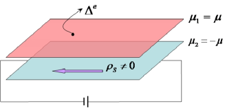
Figure 1: (color online) Schematic plot of the two Mott-Hubbard bilayer configuration. The chemical potential is chosen to have the same amount of holons in one layer as the doublons in the other. In-plane excitations in this model for doping $\delta<\delta_{c}$ (see text for definition of $\delta_{c}$) is depicted. Single-particle excitation requires a finite energy $\Delta^{e}$ due to the exciton gap. In-plane electromagnetic response is that of a superfluid even when the whole system is not a superconductor.

It proves convenient to first carry out the following particle-hole transformation of the doublon ($a=2$) layer,

$$c_{2i\sigma} \rightarrow (-1)^{i}c^{+}_{2i\sigma}$$

$$n_{2i} \rightarrow 2-n_{2i},$$ (3)

to re-write

$$H_{2} \rightarrow -t\sum_{ij\sigma}c^{+}_{2j\sigma}c_{2i\sigma}+{U\over 2}\sum_{i}(n_{2i}-1)^{2}-\mu\sum_{i}n_{2i}$$

$$H_{12} \rightarrow -V\sum_{i}(n_{1i}-1)(n_{2i}-1).$$ (4)

Due to the particle-hole transformation for $a=2$, both layers now appear as hole-doped and the inter-layer Coulomb interaction becomes attractive.

Double occupation of a given site is prohibited in the large-$U$ limit, and it is convenient to introduce the slave-boson representation of the electron operator

$$c_{ai\sigma} = b^{+}_{ai}f_{ai\sigma},$$

$$n_{ai} = 1-b^{+}_{ai}b_{ai}.$$ (5)

The constraint $b^{+}_{ai}b_{ai}+\sum_{\sigma}f^{+}_{ai\sigma}f_{ai\sigma}=1$ is included via Lagrange multiplier $\lambda_{ai}$. The slave-boson representation results in constrained hopping model for each layer:

$$H_{a} = -t\sum_{ij\sigma}b^{+}_{ai}b_{aj}f^{+}_{aj\sigma}f_{ai\sigma}+\mu\sum_{i}b^{+}_{ai}b_{ai}$$ (6)

$$+\sum_{i}\lambda_{ai}(b^{+}_{ai}b_{ai}+\sum_{\sigma}f^{+}_{ai\sigma}f_{ai\sigma}-1)$$

while the inter-layer interaction takes on

$$H_{12}=-V\sum_{i}b^{+}_{1i}b_{1i}b^{+}_{2i}b_{2i}.$$ (7)

The resulting Hamiltonian $H=H_{1}+H_{2}+H_{12}$ is solved in the slave-boson mean-field theory using the following self-consistent parameters

$$\chi^{f}=\sum_{\sigma}\langle f^{+}_{1j\sigma}f_{1i\sigma}\rangle=\sum_{\sigma}\langle f^{+}_{2j\sigma}f_{2i\sigma}\rangle$$

$$\chi^{b}=\langle b^{+}_{1j}b_{1i}\rangle=\langle b^{+}_{2j}b_{2i}\rangle$$

$$\Delta^{b}=\langle b_{1i}b_{2i}\rangle.$$ (8)

All order parameters are assumed real and uniform, and $\lambda_{ai}=\lambda$ is also assumed constant, uniform, and equal for both planes. Non-zero $\Delta^{b}$ signifies the presence of excitons formed of doublon-holon pairs across the layers. The mean-field Hamiltonian thus obtained is a sum of bosonic and fermionic parts which reads, in momentum space,

$$H^{f}_{mf} = \sum_{ak\sigma}\epsilon^{f}_{k}f^{+}_{ak\sigma}f_{ak\sigma}$$

$$H^{b}_{mf} = \sum_{ak}\epsilon^{b}_{k}b^{+}_{ak}b_{ak}-V\Delta^{b}\sum_{k}(b^{+}_{1\overline{k}}b^{+}_{2k}+b_{1\overline{k}}b_{2k}),$$

where $\overline{k}=-k$. We introduced the shorthand notation $\epsilon^{f}_{k}=\chi^{b}\epsilon_{k}+\lambda$ and $\epsilon^{b}_{k}=\chi^{f}\epsilon_{k}+\mu+\lambda$ for the renormalized fermion and boson dispersions, where $\epsilon_{k}=-2t[\cos k_{x}+\cos k_{y}]$ is the bare band dispersion appropriate for a square lattice. For later convenience we re-define $\mu$ in such a way that the boson dispersion becomes

$$\epsilon^{b}_{k}=\chi^{f}(\epsilon_{k}+D)+\mu$$

with $D=4t$ being the half bandwidth of the bare band. After carrying out appropriate Bogoliubov rotation the boson Hamiltonian is diagonalized with the quasiparticle energy $E^{b}_{k}=\sqrt{(\epsilon^{b}_{k})^{2}-(V\Delta^{b})^{2}}$.

There are two equations one can write down for the fermion and boson occupation numbers respectively, and another three for the three order parameters introduced earlier in Eq. (8). In these equations we replace the momentum sum $\sum_{k}$ by an integral $\int d\epsilon D(\epsilon)$ and use the simplistic form of the density of states $D(\epsilon)=1/(2D)$. This approximation allows us to solve the self-consistent equations analytically. Without going through the rather straightforward derivations in detail, we quote the final results of solving the five equations at zero temperature:

$$\lambda=\delta\times\chi^{b}D$$

$${1\over 2}+\delta={1\over 4\chi^{f}D}\left(\sqrt{(2\chi^{f}D+\mu)^{2}-(V\Delta^{b})^{2}}-\sqrt{\mu^{2}-(V\Delta^{b})^{2}}\right)$$

$$\chi^{f}=(1-\delta^{2})/2$$

$$\chi^{b}={1\over 2\chi^{f}D}\Bigl{(}(\mu+\chi^{f}D)(\delta+{1\over 2})-V(\Delta^{b})^{2}-{1\over 4}\bigl{(}\sqrt{(2\chi^{f}D+\mu)^{2}-(V\Delta^{b})^{2}}+\sqrt{\mu^{2}-(V\Delta^{b})^{2}}\bigr{)}\Bigr{)}$$

$$\Delta^{b}={1\over 2}V\Delta^{b}\ln\left({{1+\mu+\sqrt{(1+\mu)^{2}-(V\Delta^{b})^{2}}}\over{{\mu+\sqrt{\mu^{2}-(V\Delta^{b})^{2}}}}}\right).$$ (10)

The solution of Eq. (10) gives two phases, at $T=0$, as the doping $\delta$ is varied. For $\delta<\delta_{c}$ a featureless state is obtained with a gap in the single-particle spectrum. There is no well-defined quasiparticle peak in this regime. This phase is dubbed the spin liquid insulator, or SLI. For $\delta>\delta_{c}$ the gap closes, quasiparticle coherence recovered, and one is in the Fermi liquid (FL) regime. The critical doping $\delta_{c}$ which marks the incoherent-to-coherent crossover is zero for $V=0$ and grows as $V$ is increased. In the following we discuss the derivation of the results mentioned above. For convenience we set the overall energy scale $2\chi^{f}D$ to unity.

From the second of Eq. (10) one obtains

$$(1+2\delta)^{2}[\mu^{2}-(V\Delta^{b})^{2}]=[\mu-2\delta(1+\delta)]^{2}.$$ (11)

It is clear that self-consistency is only fulfilled for $\mu\geq V\Delta^{b}$, whereas $\mu=V\Delta^{b}$ marks the onset of Bose condensation, or BEC. Exact expressions for $\mu$ and $V\Delta^{b}$ can be found as

$$\mu = {1+\delta+\delta e^{2/V}\over e^{2/V}-1}$$

$$V\Delta^{b} = {2\sqrt{\delta(1+\delta)}e^{1/V}\over e^{2/V}-1}.$$ (12)

Note that $\mu\geq V\Delta^{b}$ according to (12). The two values coincide at the critical doping given by (restoring $2\chi^{f}D$ temporarily)

$$\delta_{c}={1\over e^{4\chi^{f}D/V}-1}.$$ (13)

The exciton amplitude $\Delta^{b}$ grows as the square root of the hole(doublon) density for small doping. The fermion part of the mean-field Hamiltonian carries no gap, but the boson spectrum has a gap equal to

$$\mathrm{min}(E^{b}_{k})=\sqrt{\mu^{2}-(V\Delta^{b})^{2}}={1+\delta-\delta e^{2/V}\over e^{2/V}-1}.$$ (14)

The gap vanishes at $\delta=\delta_{c}$.

When $\delta$ exceeds $\delta_{c}$, Bose condensation guarantees $\mu$ is fixed to $V\Delta^{b}$. For $\delta>\delta_{c}$, the residual boson density $\delta-\delta_{c}$, defined as the condensate fraction, goes into the condensate portion of the boson state. The spectral weight of the coherent quasiparticle in the $\delta>\delta_{c}$ regime grows as $\delta-\delta_{c}$. The critical doping depends on the interaction strength $V$ in the manner given in Eq. (13). It is zero for $V=0$ as expected for a single-layer Hubbard model.

The $T=0$ Green’s function for the electron in the SLI phase, $\delta<\delta_{c}$, can be worked out

$$G^{e}(k,i\omega) = \sum_{q}\cosh^{2}\theta_{q}{\theta(-\epsilon^{f}_{k+q})\over\epsilon^{f}_{k+q}-E^{b}_{q}-i\omega}$$

$$+ \sum_{q}\sinh^{2}\theta_{q}{\theta(\epsilon^{f}_{k+q})\over\epsilon^{f}_{k+q}+E^{b}_{q}-i\omega}$$

where

$$\cosh^{2}\theta_{q}={1\over 2}\left({\epsilon^{b}_{q}\over E^{b}_{q}}+1\right),~{}\sinh^{2}\theta_{q}={1\over 2}\left({\epsilon^{b}_{q}\over E^{b}_{q}}-1\right).$$

Momentum-integrated spectral function $A^{e}(\omega)$ is obtained as the imaginary part of the quantity $\sum_{k}G^{e}(k,i\omega\rightarrow\omega+i\delta)$. Evaluating the sum over $k$ as an integral with a constant density of states as before, we get the spectral function $A^{e}(\omega)$:

$${1\over 2D}\sum_{q}\cosh^{2}\theta_{q}~{}\theta(-E^{b}_{q}-\omega)\int_{-D}^{D}\delta(\chi^{b}\epsilon-E^{b}_{q}-\omega)d\epsilon$$

$$+{1\over 2D}\sum_{q}\sinh^{2}\theta_{q}~{}\theta(\omega-E^{b}_{q})\int_{-D}^{D}\delta(\chi^{b}\epsilon+E^{b}_{q}-\omega)d\epsilon.$$

The step function $\theta(-\omega-E^{b}_{q})$ appearing in the first line is non-zero only if $\omega<-E^{b}_{q}$. The step function in the second line is non-zero only if $\omega>E^{b}_{q}$. Therefore, in the range where $|\omega|<\mathrm{min}(E^{b}_{q})$ we get $A^{e}(\omega)=0$. The gap in the electronic spectral function matches that in the boson spectrum obtained in Eq. (14), establishing $\delta<\delta_{c}$ as the charge-gapped phase.

Despite the presence of the gap in the single-particle sector the SLI phase is not an electronic insulator, but a metal. It can be demonstrated by referring to the Ioffe-Larkin ruleioffe-larkin , which states that the conductivity $\sigma^{e}$ of the fermion-boson composite system is given as $(\sigma^{e})^{-1}=(\sigma^{b})^{-1}+(\sigma^{f})^{-1}$. As will be shown in the next section, the exciton pairing has a similar influence on the electromagnetic response of the bosons as the BCS pairing on fermions, and the boson conductivity $\sigma^{b}$ in the SLI phase is infinite. The fermion part is metallic, however, and the overall response of the electron system is that of a metal according to Ioffe-Larkin rule. The peculiarity arises from the bilayer nature of the model. Extracting a charge from an individual layer costs an energy gap because one has to break the exciton pair. On the other hand, in-plane motion of a holon is always accompanied by that of a doublon, which together make up an exciton that moves without an energy cost.

For $\delta>\delta_{c}$ condensation of single bosons allows us to write the coherent part of the spectral function as $A^{e}(\omega)\sim(\delta-\delta_{c})A^{f}(\omega)$ and $A^{f}(\omega)$ is constant near $\omega=0$ as in the non-interacting Fermi liquid. Therefore we have a metallic state with coherent quasiparticles for $\delta>\delta_{c}$. One can say that $\delta_{c}$ marks an incoherent-coherent crossover of the quasiparticles, while the electric transport property remains metallic for all non-zero doping.

Analysis for the second Hubbard layer is similar. Due to the particle-hole transformation (3) the electron Green’s function $\langle T_{\tau}c_{2i}(\tau)c^{+}_{2j}\rangle$ in the original model is mapped onto $-(-1)^{i-j}\langle T_{\tau}c^{+}_{2j}(\tau)c_{2j}\rangle=-(-1)^{i-j}G^{e}_{2ji}(-\tau)$ after the transformation. Likewise, the electronic Green’s function at $(k,\omega)$ is obtained as $G^{e}(Q-k,-\omega)$, $Q=(\pi,\pi)$, in the transformed Hamiltonian. However, the argument in regard to the energy gap is done summing over all available momenta $k$, so the distinction between $k$ and $Q-k$ vanishes. The second layer has a gap with the same magnitude as the first layer for $\delta<\delta_{c}$, has metallic conduction, etc.

III t-J Model Formulation

Instead of the Hubbard model in Eq. (1) we adopt the $tJ$ model for each plane:

$$H_{a}=-t\sum_{ij\sigma}c^{+}_{aj\sigma}c_{ai\sigma}-\mu_{a}\sum_{i}n_{ai}+J\sum_{\langle ij\rangle}S_{ai}\cdot S_{aj}.$$ (17)

A well-known mapping of the Hubbard model to the $tJ$ model for large $U/t$ justifies the use of $tJ$ model for the doped Mott planes. The spin-exchange term introduces additional degrees of freedom having to do with $d$-wave pairing of electrons and long-range magnetic order. We will deal with the first possibility in this section and consider the magnetic order in the next.

Under the particle-hole transformation (3) for the second layer the spin operator $(S^{x},S^{y},S^{z})$ is transformed to $(-S^{x},S^{y},-S^{z})$, but the inner product $S_{i}\cdot S_{j}$ remains unaffected. The Hamiltonian, after the particle-hole transformation is carried out, is re-written using the slave-boson substitution as the mean-field type $H_{mf}=H^{b}_{mf}+H^{f}_{mf}$ by introducing the mean-field parameters $\chi^{b}_{ij}=\langle b^{+}_{aj}b_{ai}\rangle$, $\chi^{f}_{ij}=\sum_{\sigma}\langle f^{+}_{aj\sigma}f_{ai\sigma}\rangle$, $\Delta^{b}_{i}=\langle b_{1i}b_{2i}\rangle$, and $\Delta^{f}_{ij}=\langle f_{ai\uparrow}f_{aj\downarrow}-f_{ai\downarrow}f_{aj\uparrow}\rangle$:

$$H^{f}_{mf} = -\sum_{aij\sigma}(t\chi^{b}_{ji}+J\chi^{f}_{ji})f^{+}_{aj\sigma}f_{ai\sigma}+\sum_{i}\lambda_{ai}f^{+}_{ai\sigma}f_{ai\sigma}$$

$$~{}~{}~{}-{J}\sum_{a\langle ij\rangle}(\Delta^{f}_{ij}P^{+}_{aij}+h.c.)$$

$$H^{b}_{mf} = -\sum_{aij}t\chi^{f}_{ji}b^{+}_{aj}b_{ai}+\sum_{ai}(\mu+\lambda_{ai})b^{+}_{ai}b_{ai}$$ (18)

$$-V\sum_{i}\Delta^{b}_{i}(b^{+}_{1i}b^{+}_{2i}+b_{1i}b_{2i}).$$

The fermion pairing operator is given by $P_{aij}=f_{ai\uparrow}f_{aj\downarrow}-f_{ai\downarrow}f_{aj\uparrow}$ in $H^{f}_{mf}$. Assuming all mean-field parameters are real and uniform and that the fermion gap obeys the $d$-wave symmetry, we can write down

$$H^{f}_{mf} = \sum_{ak\sigma}\epsilon^{f}_{k}f^{+}_{ak\sigma}f_{ak\sigma}-\sum_{ak}\Delta^{f}_{k}[f_{ak\uparrow}f_{a\overline{k}\downarrow}+f^{+}_{a\overline{k}\downarrow}f^{+}_{ak\uparrow}]$$

$$H^{b}_{mf} = \sum_{ak}\epsilon^{b}_{k}b^{+}_{ak}b_{ak}-V\Delta^{b}\sum_{k}[b^{+}_{1\overline{k}}b^{+}_{2k}+b_{1\overline{k}}b_{2k}]$$

$$\epsilon^{f}_{k} = \left(\chi^{b}+{J\chi^{f}\over t}\right)\epsilon_{k}+\lambda$$

$$\epsilon^{b}_{k} = \chi_{f}(\epsilon_{k}+D)+\mu$$

$$\epsilon_{k} = -2t(\cos k_{x}+\cos k_{y})$$

$$\Delta^{f}_{k} = 2J\Delta^{f}(\cos k_{x}-\cos k_{y}).$$ (19)

The self-consistent parameters $\Delta^{f}$ and $\chi^{f}$ follow from

$$\Delta^{f}=J\Delta^{f}\sum_{k}{(\cos k_{x}-\cos k_{y})^{2}\over E^{f}_{k}}$$

$$\chi^{f}=-{1\over 2}\sum_{k}(\cos k_{x}+\cos k_{y}){\epsilon^{f}_{k}\over E^{f}_{k}}$$

(20)

at zero temperature. The fermion spectrum is diagonalized with $E^{f}_{k}=\sqrt{(\epsilon^{f}_{k})^{2}+(\Delta^{f}_{k})^{2}}$. At zero doping $\epsilon^{f}_{k}$ is reduced to $-2J\chi^{f}(\cos k_{x}+\cos k_{y})$ and one readily obtains $\chi^{f}=\Delta^{f}\approx 0.33J$, as expected from SU(2) symmetry and in agreement with Kotliar and Liu’s earlier calculationkotliarliu . The hole number in each layer is given by $\delta=\sum_{k}(\epsilon^{f}_{k}/E^{f}_{k})$.

Notice that all of the boson-related self-consistent equations are identically those of the $J=0$ model derived in the previous section. The only difference arises in the numerical value of $\chi^{f}$ which enters the overall energy scale $2\chi^{f}D$. For $J=0$ we had $\chi^{f}=(1-\delta^{2})/2$, but with $J\neq 0$ it is determined self-consistently by Eq. (20). Following earlier resultskotliarliu , we anticipate that $\chi^{f}$ will remain largely constant over a wide doping range. The critical density $\delta_{c}$ is still given by Eq. (13) with appropriate $\chi^{f}$. The incoherent-to-coherent crossover in the electron spectral function with the vanishing of the single-particle charge gap occurs at this density of holes. The critical doping $\delta_{c}$ is plotted in Fig. 2 as empty squares. The fermion sector has a $d$-wave symmetry gap in the spectrum throughout the whole doping range until $\Delta^{f}$ itself vanishes at a larger doping. Therefore, $\delta_{c}$ marks the separation of the SLI from the nm-dSC (non-magnetic $d$-wave superconductor). The spectral and electromagnetic properties of the individual layer is discussed now.

The zero-temperature electronic Nambu Green’s function for the region $\delta<\delta_{c}$ is worked out as

$$G^{e}(k,i\omega) = \sum_{q}{A_{k+q}\sinh^{2}\theta_{q}\over E^{f}_{k+q}+E^{b}_{q}-i\omega}$$

$$+ \sum_{q}{B_{k+q}\cosh^{2}\theta_{q}\over E^{f}_{k+q}+E^{b}_{q}+i\omega}$$

with $A_{k}$ and $B_{k}$ given by

$$A_{k}=\left(\begin{array}[]{cc}\cos^{2}\theta_{k}&\cos\theta_{k}\sin\theta_{k}\\ \cos\theta_{k}\sin\theta_{k}&-\sin^{2}\theta\end{array}\right)$$ (24)

$$B_{k}=\left(\begin{array}[]{cc}-\sin^{2}\theta_{k}&\cos\theta_{k}\sin\theta_{k}\\ \cos\theta_{k}\sin\theta_{k}&-\cos^{2}\theta_{k}\end{array}\right)$$ (27)

$$\cos 2\theta_{k}={\epsilon^{f}_{k}\over E^{f}_{k}},~{}~{}\sin 2\theta_{k}={\Delta^{f}_{k}\over E^{f}_{k}}.$$ (28)

The corresponding spectral function contains a factor $\delta(\omega-E^{f}_{k+q}-E^{b}_{k})$ and $\delta(\omega+E^{f}_{k+q}+E^{b}_{q})$, which yields zero when $\omega=0$, provided the boson gap persists. Thus the spectral density is zero at $\omega=0$ for the SLI phase, as was the case for $J=0$. It should be noted that in regard to the single-particle gap, we no longer have the pure $d$-wave symmetry as was the case for a single-layer $tJ$ model. The existence of exciton pairing renders the gap symmetry in the SLI phase essentially that of $d+s$.

Now we present the proof that due to the exciton gap, the underdoped region $\delta<\delta_{c}$ exhibits a superfluid response to an external field. It is clear that the fermion sector behaves as a superconductor with $\sigma^{f}=\infty$ because of the $d$-wave pairing. It remains to show that the boson sector also has $\sigma^{b}=\infty$, and we would have $\sigma^{e}=\infty$ according to the Ioffe-Larkin composition rule.

The method for calculating the electromagnetic response to an electric field for a discrete lattice model had been developed earlier by Scalapino et al.scalapino . Although it was used to calculate the response properties of a fermion system, the formalism actually applies equally well to bosons. We obtain the zero-temperature superfluid density

$$\rho_{s}(T=0)={(V\Delta^{b}t\chi^{f})^{2}\over 2}\sum_{k}{\sin^{2}k_{x}+\sin^{2}k_{y}\over(E^{b}_{k})^{3}}$$ (29)

for the upper or lower plane of the bilayer. It is non-zero as long as the exciton pairing amplitude $\Delta^{b}$ persists. Except for the $(\Delta^{b})^{2}$, the rest of the terms in Eq. (29) proved to be nearly independent of doping in our numerical analysis. As a result $\rho_{s}\sim(\Delta^{b})^{2}\sim\delta$ for small $\delta$. The exciton pairing is responsible for the superfluid behavior of the bosons in each layer. The in-plane electron response in the non-superconducting SLI phase is that of a superfluid because $\sigma^{b}$ and $\sigma^{f}$ are both infinite, with $\sigma^{e}\sim\delta$ at low doping.

We note that non-zero $\Delta^{b}=\langle b_{1i}b_{2i}\rangle$ implies the total electron number in the individual layer is not conserved; rather only the sum over the two layers is. The number fluctuation within each layer is reminiscent of the similar fluctuation in the superconducting ground state and is responsible for the similar electromagnetic response.

IV t-J Model with Magnetic Order

The previous sections dealt with the physics of strongly interacting bilayers in increasing degree of complexity. First we treated the case of in-plane hopping subject only to the Mott constraint and the inter-layer Coulomb interaction that gave rise to the exciton formation. At the next level of complexity we introduced the possibility of fermion pairing and of superconducting state in each layer. In both cases we found an incoherent regime characterized by a charge gap at low doping that we called the spin-liquid-insulator, or SLI.

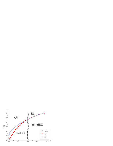
Figure 2: (color online) $\delta_{AFM}$ (black) and $\delta^{m}_{c}$ (red) for different inter-layer Coulomb interaction $V/J$ with fixed $t/J=4$ according to the mean-field decoupling scheme of section IV. The empty blue symbols are $\delta_{c}$ obtained with the magnetic moment suppressed to zero (section III). Various phases are identified: AFI (antiferromagnetic insulator), SLI (spin liquid insulator), m-dSC (antiferromagnetic $d$-wave superconductor), nm-dSC (non-magnetic $d$-wave superconductor).

In this section, the spectrum of possible phases in the bilayer system is enlarged to include the antiferromagnetic (AFM) order characterized by $m_{i}=(1/2)(-1)^{i}\langle f_{ai\uparrow}^{+}f_{ai\uparrow}-f_{ai\downarrow}^{+}f_{ai\downarrow}\rangle=m$. We consider the effects of the magnetic order on the overall phase diagram by decoupling the Heisenberg exchange interaction in the hopping, pairing, and magnetic channels. In addition to $\delta_{c}$ we have the critical concentration $\delta_{AFM}$ which marks the vanishing of magnetic order. There are four phases found, depending on the presence/absence of magnetism and of the charge gap. SLI phase, which existed for arbitrary $V$ in the previous analysis, is now only found for a sufficiently large $V/J$ and $\delta$. The low-doping region is replaced by the antiferromagnetic insulator (AFI). The superconducting phase is also distinguished by the co-existence of magnetism as the m-dSC (magnetic $d$-wave superconductor) at low doping and nm-dSC at higher $\delta$. The four phases collide at a single tetra-critical point. Below we present the details of the mean-field calculation.

Using the slave-boson substitution, the fermionic mean-field Hamiltonian $H_{mf}^{f}$ becomeshanlee

$$H^{f}_{mf} = \sum_{ak\sigma}\epsilon^{f}_{k}f^{+}_{ak\sigma}f_{ak\sigma}-\sum_{ak}\Delta^{f}_{k}[f_{ak\uparrow}f_{a\overline{k}\downarrow}+f^{+}_{a\overline{k}\downarrow}f^{+}_{ak\uparrow}]$$ (30)

$$~{}~{}~{}~{}-2Jm\sum_{k\sigma}\sigma f_{ak+Q\sigma}^{+}f_{ak\sigma}$$

where $Q$ is the AFM wave vector $(\pi,\pi)$. Other notations are identical to those used in Eq. (19). The boson mean-field Hamiltonian remains unchanged from Sec. III. Diagonalization of the fermion Hamiltonian and working out the self-consistent equations for all the parameters involved in the Hamiltonian can be done by straightforward manipulationhanlee . The self-consistent equations obtained can be solved numerically for each doping $\delta$ and a given inter-layer interaction strength $V$. As is well known from previous mean-field studieshanlee , the magnetic order vanishes at around 18% doping for a single layer $tJ$ model with $t/J=3$. In our numerical solution the critical doping concentration for the vanishing of magnetic order, $\delta_{AFM}$, does not vary greatly with $V$.

The two critical doping concentrations, $\delta_{AFM}$ and $\delta_{c}$, are worked out for varying strengths of $V$ in Fig. 2 with $t/J=4$. The value of $\delta_{c}$ obtained in the presence of magnetic order deviates from that obtained in the previous section, when magnetic order was suppressed. We use $\delta^{m}_{c}$ and $\delta^{nm}_{c}$ to differentiate the magnetic and non-magnetic critical concentrations. Both are plotted in Fig. 2. There are two new phases which were unobserved in the non-magnetic model, due to the co-existence of magnetism. The charge-gapped phase, which was SLI in the non-magnetic model, is either an AFI or SLI depending on whether the magnetic moment is non-zero or not. The $d$-wave superconducting phase also splits into non-magnetic (nm-dSC) and magnetic (m-dSC) $d$-wave superconducting phases. The magnetic phase is seen to dominate the low-doping region as expected. The spin liquid phase is pushed to high-$V/J$, high-$\delta$ region due to a competition with antiferromagnetic ordering, but still has a finite range of existence. The in-plane electromagnetic response remains that of a superfluid throughout the entire phase diagram, except in the highly doped region, not shown in Fig. 2, where $\Delta^{b}$ or $\Delta^{f}$ itself vanishes.

V Summary and Outlook

In this paper we worked out the phase diagram and some of the unique physical properties in a model of coupled Mott-Hubbard bilayers. While all the phases of a single layer model have their counterparts in the bilayer model for a sufficiently weak inter-layer interaction strength, there also exists a new phase with a gap in the single-charge excitation and incoherent quasiparticle spectra for sufficiently strong $V$ and/or $\delta$. This spin liquid insulator phase is to be distinguished from either the spin liquid obtained by frustrating the magnetic orderchandra , or the metallic spin liquid state in the high-T_c phase diagram. The uniqueness of the SLI phase we find arises from the fact that it is a charge insulator even though the doping is finite.

On the other hand, bilayer exciton formation gives rise to the superfluid electromagnetic response in each layer in the charge-gapped, spin-liquid phase. Such dichotomy of the single-particle and two-particle response functions can be explored in future experimental setup.

It will be of importance to establish the existence of the exotic SLI phase found in the present paper beyond the mean-field level and applying techniques other than slave-particle approaches. Effects of gauge fluctuations on the mean-field phases will be considered in the future work. Employing dynamical mean-field theory can help carve out the phase diagram of the model Hamiltonian used in this paper beyond the slave-particle mean-field theory.

References

• (1) A. Ohtomo, D. A. Muller, J. L. Grazul, and H. Y. Hwang, Nature (London) 419, 378 (2002).
• (2) Satoshi Okamoto and Andrew J. Millis, Nature (London) 428, 630 (2004); Phys. Rev. B 70, 075101 (2004).
• (3) J. K. Freericks, Phys. Rev. B 70, 195342 (2004); Z. S. Popovic and S. Satpathy, Phys. Rev. Lett. 94, 176805 (2005).
• (4) I. Bozovic et al. Nature (London) 422, 873 (2003).
• (5) Tiago C. Ribeiro, Alexander Seidel, Jung Hoon Han, and Dung-Hai Lee, cond-mat/0605284.
• (6) Gabriel Kotliar and Jialin Liu, Phys. Rev. B 38, 5142 (1988).
• (7) Menke U. Ubbens and Patrick A. Lee, Phys. Rev. B 46, 8434 (1992).
• (8) Douglas J. Scalapino, Steven R. White, and Shoucheng Zhang, Phys. Rev. B 47, 7995 (1993).
• (9) L. B. Ioffe and A. I. Larkin, Phys. Rev. B 39, 8988 (1989).
• (10) The details of the mean-field decoupling scheme can be found, for instance, in Jung Hoon Han, Qiang-Hua Wang, and Dung-Hai Lee, Int. J. Mod. Phys. B 15, 1117 (2001).
• (11) P. Chandra and B. Doucot, Phys. Rev. B 38, 9335 (1988).