Controllable $\pi$ junction in a Josephson quantum-dot device with molecular spin.

Abstract

We consider a model for a single molecule with a large frozen spin sandwiched in between two BCS superconductors at equilibrium, and show that this system has a $\pi$ junction behavior at low temperature. The $\pi$ shift can be reversed by varying the other parameters of the system, e.g., temperature or the position of the quantum dot level, implying a controllable $\pi$ junction with novel application as a Josephson current switch. We show that the mechanism leading to the $\pi$ shift can be explained simply in terms of the contributions of the Andreev bound states and of the continuum of states above the superconducting gap. The free energy for certain configuration of parameters shows a bistable nature, which is a necessary pre-condition for achievement of a qubit.

I Introduction

Molecular spintronics is a promising new domain, at the convergence of two challenging disciplines. On the one hand there is molecular electronics, where single molecules are used to create electronics devices at the nanometric scale with unique properties, while on the other hand there is spintronics, where the spin of the electron is used as the relevant quantity in place of the electronic charge. The latter allows us to take advantage of the unusual properties of spin, like a long coherence time. It is in this context that we consider in our work the equilibrium properties of a molecule with a large magnetic moment placed between two superconductors, when a Josephson current flows between the two superconductors through the molecule. The focus will be on the effect, on the Josephson current, of the coupling between the spin of the electrons producing the current and the molecular spin. We will show in particular that when this spin coupling is large enough, the superconducting junction behaves as a $\pi$ junction, with a reversal of the Josephson current compared to the case without spin coupling.

Of great importance for molecular spintronics are molecules possessing a large spin, or “single molecule magnets”. Such molecules can now be synthesized, for example the molecule Mn12ac, which has a ground state with a large spin $S=10$, and a very slow relaxation of magnetization at low temperature.gatteschi This slow relaxation is due to a high anisotropy barrier for the magnetization, around $5.6$ meV for Mn12ac. For the system we are considering, this is a very large energy, as the typical energies in our system (temperature, coupling to the electrodes, etc.) are at most of the order of the superconducting gap (which is $0.1$ meV in Aluminum for example). This motivates our choice to take the molecular spin as a fixed quantity, which will act as a local magnetic field for the electrons going through the molecule. Note that other systems, where the spin is not fixed, involving for example superconducting transport through fullerene molecule doped with magnetic impurities have been considered experimentally and theoretically.bouchiat05 ; levy06 Concerning the electronic transport across the molecule, we model the molecule as a single resonant level, i.e. a quantum dot. As we will be interested in the regime of good transparency between the molecules and the superconducting electrodes, we will neglect in this work the electronic interactions on the resonant level.veciono

The main result of our paper is to show that, when the coupling to the molecular spin is large enough, the system shows a $\pi$ shift. A reversal of the super-current in a Josephson device and the free energy having a global minima at phase difference $\pi$ is referred to as $\pi$ shift and a Josephson junction displaying this is termed a $\pi$ junction.golubov The $\pi$ junction has potential applications in superconducting electronics, in quantum logic circuits as switches and are an integral part of superconducting phase qubits. We will also show that this $\pi$ shift can be controlled by the other parameters of the system (position of the dot level, temperature, coupling to the electrodes, etc.), allowing to reverse the $\pi$ shift and recover a standard Josephson junction.

Generally in works related to $\pi$ junction behavior the bound state current, which is due to current carrying Andreev bound states formed between the two superconductors, is investigated while the contribution from the continuum of states above the superconducting gap is ignored.beena There are good reasons for doing so, since the continuum contribution is generally much reduced compared to bound state current, especially in the limit of a long junction or a very short one. However recent works have shown that the continuum current cannot be ignored,heikkila ; kamenev ; kirch ; jens especially in a Josephson junction which is neither very short nor very long. In this work, we calculate explicitly the contribution from the continuum, and we show that the in the presence of a large coupling to the molecular spin, the continuum current is essential to understand the $\pi$ junction behavior. In some regime, the bound state current can even vanish, and the continuum current is then the only contribution. We will show also that, with some fine-tuning of the parameters of the system, the system can be in a bi-stable state, where the $\phi=0$ and $\phi=\pi$ state are equally stable; this bi-stability is a necessary condition for a possible qubit implementation.

Figure 1: Our model system

The rest of the work is organized as follows. The next section deals with a short history of the $\pi$-shift as seen in Josephson junctions and with the possible applications which such behavior may have. Section III is devoted to the derivation of the Josephson current when coupling to the molecular spin is present. In section IV we use the formulae obtained in section III to show the behavior of the Josephson current as a function of the coupling to the molecular spin, and of the other parameters. We give a detailed explanation of the mechanism leading to the $\pi$ shift. In section V we discuss some potential applications of our system, first as a Josephson current switch, then as a superconducting qubit. Section VI is devoted to concluding remarks.

II Brief history of $\pi$-shift

In order to show how our work and results differ from existing works on $\pi$ junctions, we find useful to give a very short history of the $\pi$-shift. $\pi$ junctions were first proposed theoretically by Bulaevskii and coworkers in Ref.[Bulaevskii, ]. They considered a tunnel junction with magnetic impurities in the barrier. In this system spin-flip tunneling leads to a formation of $\pi$ junction. They also predicted that a super-conducting ring containing a $\pi$ junction could generate a spontaneous current and a magnetic flux opening the way for experimental detection. Spin flip tunneling in superconductor-quantum dot-superconductor(S-QD-S) system has also been shown to give rise to a $\pi$ junction behavior as in Refs.[glaz, ; siano, ; pan, ]. It was Kulik who in 1966 was the first to discuss the spin-flip tunneling through an insulator with magnetic impurities.kulik The spin-flip tunneling is predicted to dominate the Josephson current when spin on the quantum dot is non-zero. In S-QD-S junction, changes in the sign of the critical current could be observed as a function of the quantum dot gate voltage which controls the occupancy of a quantum dot. Due to this gating capability one has more control over the magnetic state of a barrier in S-QD-S junction compared to a magnetically doped Superconductor-Insulator-Superconductor junction.arovas Superconductor-Ferromagnet-Superconductor(SFS) have also been shown to give rise to a $\pi$ junction behavior both in theorybuzdin ; sell ; radovic as well as in experiments.ryazanov ; frolov The study of the superconducting $\pi$ state sheds more light on the coexistence of superconductivity and ferromagnetism in general and is also important for superconducting electronics.buz-baladie Generally with increase in the strength of the exchange field the $\pi$ shift is observed with a reversal and suppression of the super-current. In SFSFS systems with the ferromagnets in anti-parallel alignment, however, with increase in the strength of the exchange field an increase in super-current is observed.bergeret In SIFIS and SFcFS, where c denotes a constriction, structures also such $\pi$ junctions have been observed.golubov Recently triplet superconductor-ferromagnet-triplet superconductor junctions have been predicted to have potential applications as current switches.boris In contrast to SFS systems, $\pi$ junction behavior in SNS systems occurs due to the creation of a non-equilibrium distribution of electrons in the barrier via a control channel.baselmans Thus in these systems the $\pi$-junction can be controlled via a voltage applied to the control channel this makes such devices ideal for them to be used in superconducting digital circuits, especially as a phase inverter, i. e., $\pi$-SQUIDguichard for complementary Josephson digital devices. Further application of $\pi$ junctions as candidates for engineering quantum bits have been predicted.ioffe Finally, $\pi$ junctions have also been theoretically predicted and experimentally observed in superconducting d-wave junctions.golubov

III Derivation of the Josephson current

III.1 Model Hamiltonian

The Josephson Current($I_{J}$) can be calculated from the derivative of the free energy(F) with respect to the phase difference($\phi$) across the superconducting leads $I_{J}=2\frac{dF}{d\phi}$, in equilibrium. The free energy in turn is defined as $F=-kT\ln Z$, where Z is the partition function of our system. Thus calculating Z is the first step in calculating the Josephson current in our system. The full Hamiltonian of our system is written as below:

$$H=H_{D-S}+\sum_{j=L,R}H_{j}+H_{T},$$ (1)

where $H_{D-S}$ defines the Hamiltonian of the quantum-dot molecule with spin, $H_{j}$ represents the superconducting leads, while $H_{T}$ denotes the tunneling part. The dot-spin Hamiltonian is:

$$H_{D-S}=\epsilon\sum_{\sigma}d_{\sigma}^{\dagger}d_{\sigma}+JS(d_{\uparrow}^{\dagger}d_{\uparrow}-d_{\downarrow}^{\dagger}d_{\downarrow})$$ (2)

where $d_{\sigma},d_{\sigma}^{\dagger}$ are the electronic operators in the dot, $\epsilon$ is the energy level of the dot, $J$ the coupling between the molecular spin ${\bf S}$ and the electronic spin on the dot level. The coupling term comes from the exchange interaction $J{\bf S}\cdot{\bf s}$, where ${\bf s}$ is the electronic spin on the dot, but as explained in the introduction, the molecular spin is fixed in our system, and we chose the spin quantization axis along the spin orientation. In the superconducting Hamiltonian it is convenient to perform a gauge transformation which removes the phase from the order parameter.schrieffer Thus,

$$H_{j}=\sum_{k}\Psi_{jk}^{\dagger}(\xi_{k}\sigma_{z}+\Delta\sigma_{x})\Psi_{jk},\Psi_{jk}=\left(\begin{array}[]{c}\psi_{jk,\uparrow}\\ \psi_{j(-k),\downarrow}^{\dagger}\end{array}\right)$$ (3)

and finally the tunnelling part can be written in the standard form with a hopping parameter $t_{j}$ determining the transfer properties of the junction. The Pauli matrices mentioned in the above equation are matrices in particle-hole space. The effect of the gauge transformation on the tunnel Hamiltonian is the appearance of a phase dependence in the hopping parameter

$$H_{T}=\sum_{jk}\Psi_{jk}^{\dagger}T_{j}d+h.c.,\quad\quad d=\left(\begin{array}[]{c}d_{\uparrow}\\ d_{\downarrow}^{\dagger}\end{array}\right)$$ (4)

with $T_{L}=t_{L}\sigma_{z}e^{i\sigma_{z}\phi/4},T_{R}=t_{R}\sigma_{z}e^{-i\sigma_{z}\phi/4}$, where $\phi$ is the phase difference between the superconducting leads, and $t_{j}$ is the tunnelling amplitude between the $j$th lead and dot.

III.2 Neglecting Coulomb interaction

In the present work we chose to neglect the charging energy of the molecule. Molecular electronics transport calculations are typically concerned with two limits: either the limit where the tunnelling rate from the molecule to the leads dominates over the charging energy, or the opposite limit of strong Coulomb blockade which can be dealt in the incoherent regime or in the coherent regime. The validity of each regime depends on the transparency of the tunnel barriers connected to the molecule, and on the capacitances seen by the molecular quantum dot with respect to the leads. So far in the literature, many efforts have focused on the Landauer-Buttiker description of molecular electronics transport. landauer_buttiker In some instancesfagas this approach is supplemented by taking Coulomb interactions in an effective manner using density functional theory, but the Green function which is used to compute the transmission coefficient is determined from a specific electron configuration, as for an effective one-electron Coulomb potential. Here we adopt a Hamiltonian approach to compute the current, but the basic assumptions for neglecting Coulomb blockade effects also apply. This is justified as follows.

In fact this stems from the fact that the charging energy of the molecular quantum dot is assumed to be small compared to the the escape rate of the electrons from the dots to the leads, later to be referred to as $\Gamma$. This regime triggers a substantial broadening of the dot level, as for instance was discussed in Ref.[guyon_mujica, ] where a molecule was attached to metallic substrate, being effectively “metalized”. Qualitatively speaking, if the transparency from the dot to the leads is close to unity, the time scale which characterizes the lifetime of electrons on the molecular quantum dot is so short that Coulomb blockade effects do not have time to operate.

These qualitative arguments are substantiated by theoretical works on the Coulomb blockade in the presence of highly transmissive barriers, which were carried out more than a decade ago. Ref.[flensberg, ] studies the behavior of a quantum dot embedded between two point contacts, and finds a crossover to a regime where charge fluctuations in the dot are dominant, therefore wiping out charge quantization (Coulomb blockade) effects. The temperature which characterizes this crossover is of course proportional to the dot charging energy, but it also goes to zero in the limit of ideal transmission. Ref.[matveev, ] considers a quantum dot connected to single barriers, and shows that the energy of the dot undergoes (Coulomb blockade) oscillations as a function of gate voltage as long as the transmission coefficient of the barrier, which isolates the dot, does not approach unity. On another note, Ref.[nazarov, ] uses a path integral frameworkschon_zaikin to describe a quantum dot with arbitrary barriers. Previous resultsflensberg concerning charge fluctuations are recovered, but more importantly it is shown that the effective charging energy is exponentially reduced at ideal transmission. This latter result applies, granted to a dot coupled to several channels, but these features are expected to survive for a a dot coupled to a single, highly transmissive channel.

Note that in the above, it is sufficient for only one of the two contacts to have a large capacitance in order to be able to neglect Coulomb effects. The present point of view is consistent with recent works on molecular electronics issues where phonons are involved other_no_coulomb , but electron-electron interactions are neglected nevertheless.

Finally, we stress the fact that there exist actual experiments in molecular electronics, which can achieve the high transmission conditions which are assumed in the present work. It has been demonstrated that break junction geometriesruitenbeek can achieve close to ideal transmission: for a Hydrogen molecule which is sandwiched between Platinum electrodes, one observes a conductance quantization plateau at $2e^{2}/h$, when bringing the two electrodes together, as expected from a monovalent metal as Hydrogen (in contrast, a pure platinum junction yields steps at $4e^{2}/h$). This is the direct evidence of single, perfectly transmitting channel. To summarize, in these works, which have been extended to study the effects of vibrations on the moleculeruintenbeek2 , no Coulomb blockade effects show up at all. For the present study, we thus assume that our molecule is placed under the same conditions as in these break junction experiments. Note that high transmission conditions have also been obtained with Carbon nanotubesbouchiat99 ; bouchiat01 .

III.3 Effective action

To calculate the partition function we use the path integral approach. In this method the partition function is given by:

$$Z=\int\prod_{jk}(\mathcal{D}{\bar{\Psi}_{jk}}\mathcal{D}{\Psi_{jk}}\mathcal{D}{\bar{d}}\;\mathcal{D}{d})\;e^{-S_{A}}$$ (5)

Z is written as a functional integral over grassmann fields for the electronic degrees of freedom ($\Psi,\bar{\Psi}$). The Euclidean action reads:

$$S_{A}=S_{D}+\int_{0}^{\beta}\!d\tau[\sum_{jk}{\bar{\Psi}_{jk}(\tau)}(\partial_{\tau}+\xi_{k}\sigma_{z}+\Delta\sigma_{x})\Psi_{jk}(\tau)+{H_{T}(\tau)}]$$

$\beta$ is the inverse temperature, and ${H_{T}(\tau)}=\sum_{jk}{\bar{\Psi}_{jk}(\tau)}T_{j}d(\tau)+h.c.\mbox{ while }S_{D}=\int_{0}^{\beta}\!d\tau[{\bar{d}}(\partial_{\tau}+\epsilon\sigma_{z}+JS)d]$. After integrating out the leads we get

$$Z=\int\!\mathcal{D}{\bar{d}}\;\mathcal{D}d\;e^{-S_{eff}}\quad\mbox{with}\quad\quad S_{eff}=S_{D}-\int_{0}^{\beta}\!d\tau\;d\tau^{\prime}\;{\bar{d}(\tau)}{\check{\Sigma}(\tau-\tau^{\prime})}d(\tau^{\prime})$$ (6)

where $\check{\Sigma}(\tau)=\sum_{j=L,R}T_{j}^{\dagger}G(\tau)T_{j}$ and $G(\tau)=\sum_{k}(\partial_{\tau}+\xi_{k}\sigma_{z}+\Delta\sigma_{x})^{-1}\delta(\tau)$.

We perform a Fourier transform on the Matsubara frequencies (with $w_{n}=(2n+1)\pi/\beta$): $\delta(\tau)=\frac{1}{\beta}\sum_{w_{n}}e^{-iw_{n}\tau}$ and $G(\tau)=\frac{1}{\beta}\sum_{w_{n}}e^{-iw_{n}\tau}G_{w_{n}}$, which gives for the Green function $G$:

$$G_{w_{n}} = \int\!d\xi\;\nu(\xi)(-iw_{n}+\xi_{k}\sigma_{z}+\Delta\sigma_{x})^{-1}\simeq\frac{\pi\nu(0)}{\sqrt{w_{n}^{2}+\Delta^{2}}}(iw_{n}+\Delta\sigma_{x})$$ (7)

In the above equation, $\nu(\xi)=\sum_{k}\delta(\xi-\xi_{k})$ is approximated as a constant $\nu(0)$, the density of states at the Fermi level in the normal leads. This gives for the self-energy:

$${\check{\Sigma}_{w_{n}}}=\frac{{\Gamma/2}}{\sqrt{\Delta^{2}-(iw)^{2}}}[iw_{n}-\Delta\cos(\phi/2)\sigma_{x}-\gamma\Delta\sin(\phi/2)\sigma_{y}]$$ (8)

with $\gamma=\frac{\Gamma_{L}-\Gamma_{R}}{\Gamma_{L}+\Gamma_{R}},{\Gamma}=\Gamma_{L}+\Gamma_{R},\Gamma_{L/R}=2\pi\nu(0)t_{L/R}^{2}$. We get finally for the effective action (introducing $d(\tau)=\frac{1}{\sqrt{\beta}}\sum_{w_{n}}e^{-iw_{n}\tau}d_{w_{n}}$)

$$S_{eff}=\sum_{w_{n}}\bar{d}_{w_{n}}{\cal M}_{w_{n}}d_{w_{n}}\quad\mbox{with}\quad{\cal M}_{w_{n}}=-iw_{n}+\epsilon\sigma_{z}+JS-{\check{\Sigma}_{w_{n}}}$$ (9)

III.4 Andreev Levels

The dispersion equation for the Andreev levels is given by the eigenvalues of the effective action in Eq. (9) (with $iw=z$)

$$\det\left[z-\epsilon\sigma_{z}-JS+\frac{\Gamma/2}{\sqrt{\Delta^{2}-z^{2}}}(z-\Delta\cos(\phi/2)\sigma_{x}-\gamma\Delta\sin(\phi/2)\sigma_{y})\right]=0$$ (10)

which gives (introducing the parameter $s=JS$):

$$(z+\frac{\Gamma z}{2\sqrt{\Delta^{2}-z^{2}}}-\epsilon-s)(z+\frac{\Gamma z}{2\sqrt{\Delta^{2}-z^{2}}}+\epsilon-s)-\frac{\Gamma^{2}\Delta^{2}(\cos^{2}(\phi/2)+\gamma^{2}\sin^{2}(\phi/2))}{4(\Delta^{2}-z^{2})}=0$$ (11)

While this cannot be solved analytically in general, there are two limiting regimes where one can get an analytical expression of the solutions, giving two Andreev levels. For simplicity, we choose here $\epsilon=0$ and $\gamma=0$.
case 1: ${\Gamma}\gg\Delta:$

$$z=E_{1,2}=\Delta\,\cos\left[\mbox{Arccos}\left(\frac{\pm\cos{\phi/2}}{\sqrt{1+4s^{2}/\Gamma^{2}}}\right)+\mbox{Arctan}\left(\frac{2s}{\Gamma}\right)\right]$$ (12)

case 2: ${\Gamma},s\ll\Delta:$

$$z=E_{1,2}=s\pm\frac{\Gamma}{2}\cos(\phi/2)$$ (13)

In the general case, for arbitrary $\Gamma,\epsilon,s(=JS)$ and $\Delta$, we calculate numerically the roots, by transforming the l.h.s. of Eq. (11) into a 8th order polynomial in z to get rid of the square roots, and then calculating the roots of this polynomial. We find that only two of these roots correspond to roots of Eq. (11) (see also ref. [kirch, ]), and that these two roots are real and belong to $[-\Delta,\Delta]$. There are thus always two Andreev bound states, as in the zero spin case: the effect of the spin term is merely to move these two states, but it does not introduce new bound states.

In Fig. 2, we plot the two Andreev bound state positions as a function of the phase difference for four values of spin, $|s|=0,1,2,$ and $4$, for large transparency of the contacts ($\Gamma=4.0$) and very low temperature ($\beta=1000$). $\Delta=1$ is taken as the unit of energy in our system, as in the rest of this work. The right panel in Fig. 2 corresponds to $s>0$ while left panel is for $s<0$. We see that when the absolute value of $s$ is increased, the two Andreev levels are pushed towards $+\Delta$ or $-\Delta$.

It might seem surprising that the Andreev bound states are different for $+s$ and $-s$. Indeed, our physical system is invariant under the interchange of spin up and spin down electron combined to the exchange $s\to-s$; as the superconductors are the same under the spin interchange, our physical system has thus to be invariant under the transformation $s\to-s$. As will be shown in the next sections, the total Josephson current, which is a physically measurable quantity, is invariant under this transformation ($s\to-s$). However, the expression of this total current in terms of the Andreev bound state current and of the continuum current, depends on ths sign of $s$ (and so do the Andreev bound states). jens

The different Andreev bound states obtained for $s$ and for $-s$ are thus two different ways to represent the same physical situation. The fact that we obtain one of the two possibilities for a given external spin can be traced back to our initial choice of the spinors for the superconductors (Eq. (3)) and for the dot (Eq. (4)): had we chosen the spinors defined with opposite spin (for example, $d^{\dagger}=(d^{\dagger}_{\downarrow},d_{\uparrow})$, to be compared with the definition of Eq. (4)), we would have obtained for $s<0$ the Andreev bound states shown here for $s>0$, and vice-versa. One could also use a combination of the two possibilities of spinors, in order to get a spectrum of Andreev bound states (and bound state current) which is independent of the sign of $s$; in this case, the spectrum is composed of four Andreev bound states, which are precisely the two we obtained for $s>0$ plus the two for $s<0$. In this paper, we have chosen to keep the spinors as defined in Eq. (3) and Eq. (4). This choice will give us a particularly simple picture for the mechanism leading to the pi-shift (see below).

Figure 2: The two Andreev bound states as function of phase difference. For $s>0$ in the right panel and for $s<0$ in the left panel. The labelling of the curves is as follows: spin s=0(black,solid line), 1.0 (red,dotted line), 2.0 (blue,dashed line) and 4.0 (green, dot-dashed line). The other parameters are $\Gamma=4.0$, $\gamma=0.0$, $\beta=1000$, $\epsilon=0.0$, and $\Delta=1.0$.

III.5 Josephson Current

The partition function after integrating out the $\{d,{\bar{d}}\}$ variables is given by-

$$Z=\int\!\mathcal{D}{\bar{d}}\;\mathcal{D}d\;e^{-S_{eff}}=\prod_{w_{n}}\det{\cal M}_{w_{n}}$$ (14)

where ${\cal M}_{w_{n}}$ is given in Eq. (9). The Josephson current then reduces to:

$$I_{J} = -\frac{2}{\beta}\frac{\partial}{\partial\phi}\ln Z=-\frac{2}{\beta}\frac{\partial}{\partial\phi}\sum_{w_{n}}\ln(\det{\cal M}_{w_{n}})$$ (15)

$$= -\frac{1}{\beta}\sum_{w_{n}}\frac{\Gamma^{2}\Delta^{2}(1-\gamma^{2})\sin(\phi)}{4[\det{\cal M}_{w_{n}}](\Delta^{2}-(iw_{n})^{2})}=-\frac{1}{\beta}\sum_{w_{n}=-\infty}^{\infty}f(iw_{n})$$

where the last equality defines the function $f$.

Further, the Free energy is given by:

$$F=-\frac{1}{\beta}\sum_{w_{n}}\ln(\det{\cal M}_{w_{n}}).$$ (16)

In the above equations, $\det{\cal M}_{w_{n}}$ is the same as the l.h.s of Eq. (11), with $iw_{n}$ replacing $z$.

¿From the above equation, one can calculate the total Josephson current by summing over the Matsubara frequencies. However, we can transform the above equation in order to separate explicitly the contributions of the Andreev bound states and of the continuum, which are physically meaningful. In order to calculate these contributions, we take advantage of the fact that the Matsubara frequencies are the poles of the Fermi function $n_{f}(z)$ [mahan, ]. We then consider the integral $I=\int_{C}\frac{dz}{2\pi i}f(z)n_{f}(z)$, where the function $f(z)$ is defined in Eq. (15). The function $f(z)$ as seen earlier has two poles on the real axis between $-\Delta$ and $\Delta$ (these are simply the two Andreev bound states, for which $\det\mathcal{M}=0$). Further, because of the square roots terms in the $\det\mathcal{M}$, it has branch points at $z=\pm\Delta$; we have chosen to place branch cuts on the real axis, for $z\in[\Delta,\infty]$ and $z\in[-\infty,-\Delta]$. We thus chose the contour C as two large semi-circles plus parts going around the branch cuts. We illustrate the contour, poles and branch cuts in Fig. 3. Thus integral I can be broken into the sum of the contributions from the large circle $D$ of radius $R$, the two small circles at $\pm\Delta$, denoted by $d_{1,2}$ of radius $\epsilon$, and the contribution from the branch cuts. Therefore,

$$I=\frac{1}{2\pi i}\int_{C}f(z)n_{f}(z)dz = \frac{1}{2\pi i}\int_{D}\!\!dz\;f(z)n_{f}(z)+\frac{1}{2\pi i}\int_{d_{1}}\!\!dz\;f(z)n_{f}(z)+\frac{1}{2\pi i}\int_{d_{2}}\!\!dz\;f(z)n_{f}(z)$$ (17)

$$+ \frac{1}{2\pi i}\lim_{\epsilon\rightarrow 0}\int_{\Delta}^{\infty}\!\!\!\!dz\;[f(z+i\epsilon)-f(z-i\epsilon)]n_{f}(z)$$

$$+ \frac{1}{2\pi i}\lim_{\epsilon\rightarrow 0}\int_{-\infty}^{-\Delta}\!\!\!\!dz\;[f(z+i\epsilon)-f(z-i\epsilon)]n_{f}(z)$$

The integrals over $D$ and $d_{1,2}$ tend to zero as $R\rightarrow\infty$ and $\epsilon\rightarrow 0$. The last two terms in the above equation define the contribution from the continuum to the current, which we denote as $I_{c}$.

Figure 3: The contour includes poles from the Fermi function, two Andreev bound states and the contribution from the branch cuts.

From Cauchy’s residue theorem the integral I can also be evaluated as follows:
(a) Function $n_{f}(z)=\frac{1}{e^{\beta z}+1}$ has poles at $z=iw_{n}$, with residue $-1/\beta$. The contributions from these poles is thus: $-\frac{1}{\beta}\sum_{w_{n}}f(iw_{n})$, which is precisely $I_{J}$ (Eq. (15)).
(b) $f(z)$ has 2 poles of its own, written $E_{1}$ and $E_{2}$. These gives the Andreev bound states contribution, which we denote by $I_{b}$.
We have thus

$$\left\{\begin{split}I_{J}&=I_{b}+I_{c}\\ I_{b}&=-n_{F}(E_{1})\mbox{res}(f(E_{1}))-n_{F}(E_{2})\mbox{res}(f(E_{2}))\\ I_{c}&=\lim_{\epsilon\rightarrow 0}\frac{1}{\pi}\left[\int_{\Delta}^{\infty}\!\!dz+\int_{-\infty}^{-\Delta}\!\!dz\right]\Im(f(z+i\epsilon)n_{f}(z+i\epsilon))\end{split}\right.$$ (18)

where res denotes the residue of the quantity in square brackets, and $\Im$ stands for the imaginary part. We see from the equation giving $I_{b}$ that the contribution from each Andreev bound state is simply proportional to the occupation number $n_{F}(E_{i})$ $(i=1,2)$ of this level. Equation (18) is the central result of this work, which we have used to calculate numerically the $I_{b}$ and $I_{c}$ curves shown in the following.

IV Results

In this section, we show the results obtained numerically for the Josephson current using equation (18). We will see that, when the coupling to the spin is strong enough, the junction behaves as a $\pi$ junction, and that the other parameters of the system allow a control of this $\pi$ junction. We will also show that the mechanism leading to this $\pi$ junction behavior can be understood simply in terms of the bound states and continuum contributions to the Josephson current.

IV.1 Total Josephson current and free energy: The $\pi$ shift

In Fig. 4, we plot the Josephson current($I_{J}$) as a function of the phase $\phi$, for different values of the spin coupling $s=JS$. We clearly see a $\pi$-junction type behavior as the magnitude of the spin coupling is increased. One clear inference from Fig. 4 is that the strength of the spin coupling required to engineer a $\pi$ junction behavior increases with the interface transparency $\Gamma$. We get another point of view of this $\pi$ shift in Fig. 5, where we plot the free energy $F$ as a function of the phase $\phi$. We see that with increase in spin coupling strength the transition from the $0$ to the $\pi$ phase is clearly marked: the absolute minimum of $F$ shifts from $\phi=0$ to $\phi=\pi$.

This figure also brings out other features, namely the $0^{\prime}$ and $\pi^{\prime}$ phases. As is evident from Fig. 5, the labelling of the respective junctions as $0,0^{\prime},\pi^{\prime}$ and $\pi$ configurations, follows from the respective stability of $\phi=0$ and $\phi=\pi$ configurations. For a $0(\pi)$ junction, only $\phi=0(\phi=\pi)$ is a minimum of $F(\phi)$. For the other two cases, both $\phi=0,\pi$ are local minima and depending on whether $\phi=0(\phi=\pi)$ is the global minimum, one has a $0^{\prime}(\pi^{\prime})$ junction.arovas Of particular interest is the bistable junction, in which both $\phi=0$ and $\phi=\pi$ are global minima; note that this bi-stability is a necessary precondition for the realization of a Josephson junction qubit.ioffe

The total Josephson current and the free energy are invariant with respect to the change of sign of the spin ($s\to-s$). As explained in part B of the previous section, this is to be expected from the invariance of the system under the spin up - spin down exchange. Technically, it can be seen on Eqs. (15)-(16), using $\omega_{-(n+1)}=-\omega_{n}$. Note that, as explained before, the Andreev bound states are not invariant under $s\to-s$, and thus the Andreev bound states current and the continuum current are also not invariant.

Figure 4: The total Josephson current ($I_{J}$)as function of the phase difference for increasing spin. The $\pi$ junction behavior is clearly seen. (a) $\Gamma=0.2$. (b)$\Gamma=2$. (c)$\Gamma=10$. The other parameters are: $\Delta=1.0,\beta=1000,\gamma=0,$ and $\epsilon=0$.

Figure 5: The Free energy (F) as function of the phase difference ($\Phi$) for increasing spin from top to bottom. The $\pi$ junction behavior is clearly seen. The other parameters are: $\Delta=1.0,\Gamma=4.0,\gamma=0,\beta=1000$ and $\epsilon=0$.

IV.2 Mechanism of the $\pi$-shift

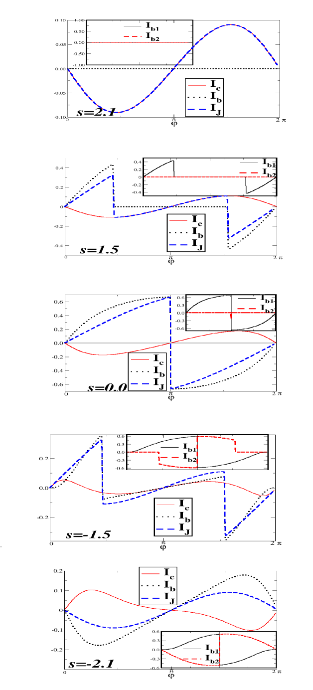
Figure 6: The Andreev bound state current ($I_{b}$), continuum current ($I_{c}$) and total Josephson current ($I_{J}$) as function of phase difference $\phi$. The individual Andreev bound state contributions ($I_{b1},I_{b2}$) are plotted in the insets. Central figure is for spin $s=0.0$. The two figures to the bottom of the central figure depict the case of $s<0$, the first is for spin $s=-1.5$ and last one on the bottom is for $s=-2.1$. On the top of the central figure the two figures depict the case of $s>0$. The individual figures plotted are for spin $s=1.5$ and lastly for $s=2.1$. The other parameters are: $\Delta=1.0,\Gamma=4.0,\gamma=0.0,\beta=1000$ and $\epsilon=0$.

The ability to distinguish, in the Josephson current, between the contributions from each Andreev bound state and from the continuum (see Eq. (18)) provides us with a simple picture for the mechanism leading to the $\pi$ shift for large spin coupling. Note that the picture we obtain depends on the initial choice of spinors (see the discussion at section III D); the choice we make here allows us to get a very simple picture. In a few words, the effect of the spin coupling is to reduce or suppress the Andreev bound states contribution, and to give more importance to the continuum contribution, and this leads to the $\pi$ shift. With more details, the effect of the spin coupling on the bound states current can be understood from Eq. (18) and Fig. 2. For $s=0$, we see in Fig. 2 that there is always one bound state below the Fermi level, and the other one above. As the contribution of a bound state to the Josephson current is proportional to the occupation number $n_{F}(E_{i})$ of this bound state (Eq. (18)), this means that we have only one bound state contributing to the current, and this contribution appears to be much larger than the continuum contribution. With a large positive spin coupling $s$, we see on Fig. 2 that both Andreev bound states are above the Fermi level, which means their contribution to the Josephson current vanishes; while for a large negative spin coupling $s$, we see that both bound states are below the Fermi energy, which means they both contribute to the Josephson current, and this reduces the total bound state contribution as the respective contributions of the two bound states have opposite signs. Note that the total Josephson current is independent of the spin coupling sign, but that for large $s>0$ there is only the contribution from the continuum, while for large $s<0$ there is a combinations of the bound states and the continuum contributions. This explanation is illustrated on Fig. 6, where the contributions of the bound states and of the continuum are plotted for different values of $s$.

The origin of the continuum current -which is non-zero even at zero temperature- is due to the phase difference between the two superconductors, which breaks the symmetry between the left and right-moving quasi-particles.bagwell92 ; continuum One can draw an analogy with persistent currents flowing in normal metal rings at zero temperature. In normal metal rings the flux breaks the symmetry between clockwise and anti-clockwise moving electrons inducing the persistent current. At zero temperature all states below the Fermi energy are filled, still then the persistent current is non-zero.buttiker

We also observe that the continuum current generally flows opposite to the bound state current. This observation is in agreement with that of other works.kamenev ; kirch

We finally add that one can also understand the fact that the full current is the same for $+s$ and $-s$ but with different contributions from bound states and continuum by using electron hole symmetry. At first sight, electron hole symmetry only holds when the dot level coincides with the superconducting chemical potential. We first discuss this case, and then we address below the case where a gate voltage shifts the dot level away from this location.

Consider the case of negative coupling ($s<0$) in Fig. 2a. From the electron point of view, occupied states below the Fermi level have a continuum contribution to the current and a bound state contribution. From the point of view of holes, which occupy all states above the Fermi level, there is a continuum contribution to the current of occupied hole states while the contribution of bound states above the Fermi level diminishes with increasing $|s|$. For sufficiently large $|s|$, the two bound states are below the Fermi level and the holes cease to have a bound state contribution. On the opposite, for positive coupling in Fig. 2b, the role of electrons and holes is reversed: from the electron point of view, the bound state contribution is reduced –and eventually vanishes – when increasing $s>0$; from the hole point of view, holes occupying both the continuum and the Andreev bound states above the Fermi level. We thus see that for positive (negative) $s$, the role of electrons and holes is reversed, and the electron hole symmetry can explain why physically observable quantities are invariant under the substitution $s\to-s$.

Next consider the case where the dot level does not coincide with the chemical potential ($\epsilon\neq 0$). In any normal metal devices, this indeed breaks electron hole symmetry, nevertheless we wish to point out that because we are dealing with a superconducting system the above argumentation still holds. When dealing with an arbitrary superconductor-normal metal- superconductor (SNS) junction, Andreev bound states are understood from the conversion of electrons into holes and vice versa at the superconducting junction. An alternative picture is to say that two electrons, one above the chemical potential with energy $E$, and one below with energy $-E$ are transfered through the normal region from one superconductor to the other. For our quantum dot setup, calculations of the Josephson current could for instance be performed using T-matrix formalism (to all orders for an exact result), where information about energies appears only in the form of differences of energy levels ($E-\epsilon$ for the positive energy electron and $E+\epsilon$ for the negative energy electron). These two energy differences are invariant under the change $\epsilon\to-\epsilon$. A dot with say, $\epsilon>0$ will thus have the same Andreev bound states spectrum and Josephson current, as a dot with $\epsilon<0$. This is indeed explicit in Eq. (11), which is invariant under the transformation $\epsilon\to-\epsilon$. In the presence of the impurity spin the bare dot level is split by a Zeeman like coupling (the exchange term), nevertheless the above statement ($\epsilon\to-\epsilon$ symmetry in the energy differences) still applies: the Andreev spectrum is reversed between $+s$ and $-s$, but the Josephson current is shown to be the same because it can be computed from the point of view of electrons (say, for $+s$) or, alternatively, of holes (for $-s$).

In conclusion, because the Andreev bound state is the same for positive and negative $\epsilon$, the symmetry $+s\to-s$ also holds for physically observable quantities such as the current. The argument for $\epsilon=0$ describing the contribution of electrons and holes populations on the continuum and discrete levels is unaffected by the modification $\epsilon\neq 0$. This fact is demonstrated in Fig. 7c, where the bound state spectrum is plotted as a function of flux for several values of $\epsilon$, for positive and negative $s$.

IV.3 Controlling the $\Pi$ shift

Figure 7: (A) The Andreev bound state current ($I_{b}$, dotted line), the continuum contribution ($I_{c}$, solid line) and the total Josephson current ($I_{J}$, dashed line) as function of dot level $\epsilon$, for positive coupling. The $\pi$ junction behavior is clearly seen as dot level is varied, in the insets the individual bound state contributions($I_{b1},I_{b2}$) are plotted for $s<0$ and positive $s>0$ (for $s<0$ the continuum and total bound state currents are also plotted). The total Josephson current ($I_{J}$) is identical for $s<0$ and $s>0$. The other parameters are: $\Delta=1.0,s=2.1,\phi=\pi/2,\Gamma=4.0,\beta=1000$ and $\gamma=0$. (B) The Free energy as function of the phase difference ($\phi$) for increasing dot energies, and (C) Andreev levels for both negative as well as positive coupling. The other parameters for B and C are: $\Delta=1.0,s=2.1,\Gamma=4.0,\beta=1000$ and $\gamma=0$.

Figure 8: (A) Andreev bound state current ($I_{b}$), the continuum contribution ($I_{c}$) and the total Josephson current ($I_{J}$) as function of inverse temperature $\beta$ for positive coupling. The $\pi$ junction behavior is clearly seen as inverse temperature $\beta$ is varied. In the insets the individual bound state currents for the case of $s>0$ and $s<0$ are plotted. For $s<0$, the continuum along with the total bound state current is also plotted. The total Josephson current $I_{J}$ is identical for $s>0$ and $s<0$. The other parameters are: $\Delta=1.0,s=2.1,\epsilon=0.0,\gamma=0.0,\phi=\pi/2$ and $\Gamma=4.0$.(B)The Free energy as function of the phase difference at different temperatures. The junction is bistable at the crossover between $0-\pi$ junction behaviors. The other parameters are: $\Delta=1.0,s=2.1,\epsilon=0.0,\gamma=0.0,$ and $\Gamma=4.0$.

A remarkable feature of our system is that the $\pi$ shift behavior can be controlled and reversed using the different parameters of the system. This is important for potential experimental implementations, as some of these parameters can be accessed relatively easily (one can for example move the dot level by using a gate voltage park ), while the spin coupling is a fixed quantity which depends in the molecule used. Our results show that, when the spin coupling is large enough to have a $\pi$ junction, a change in any of the parameter of the system (dot level $\epsilon$, coupling to the leads $\Gamma$, asymmetry of this coupling $\gamma$, and even the temperature) makes it possible to have the system behave as a standard $0$ junction (going through any intermediate situation between $\pi$ and $0$ junction). Schematically, the mechanism for this can be understood along the same lines as the explanation given above for the $\pi$ shift: starting from a $\pi$ junction situation, where both Andreev levels are (for example) above the Fermi energy and thus do not contribute to the Josephson current, changing a parameter of the system can move the Andreev level positions, and as soon as one of the Andreev level goes below the Fermi energy, it gives an important bound state contribution which brings the system back to a $0$ junction behavior. This is illustrated on Fig. 7, where the dependence of the currents (panel A), of the free energy (panel B) and of the Andreev levels (panel C) as a function of the dot level position $\epsilon$. Similar plots are obtained when looking at the $\Gamma$ or $\gamma$ dependence (not shown).

The picture is a bit different when the temperature is changed, as there the Andreev levels do not move, but the Fermi functions become broader as temperature is increased, leading to a partial revival of the bound state current. This is shown on Fig. 8, where the dependence of the currents (panel A) and of the free energy (panel B) is shown as a function of $\beta=1/(k_{B}T)$. Starting from low temperature (high $\beta$), with a $\pi$ junction behavior (the total current $I_{J}$ is $<0$, and the free energy has its minimum at $\phi=\pi$), we see that when the temperature increases ($\beta$ decreases), the total current becomes positive, and the minimum of the free energy shifts from $\phi=\pi$ to $\phi=0$.

V Discussion

We have studied in the previous sections the behavior of the Josephson current as a function of the spin coupling strength, and found that a $\pi$ junction behavior appears when this coupling is large enough. In view of an experimental realization, one must ask if the actual value of the spin coupling obtained with a given molecular magnet is large enough to observe this $\pi$ junction behavior. While a precise estimate, for a real molecule, of the magnetic coupling energy between the electronic spin and the molecular spin is beyond the scope of this paper, we can get a gross estimate by calculating the interaction energy of two magnetic dipoles at a distance typical of the molecular distance involved in our problem. Taking a spin $S=10$ for the molecule (as in Mn12ac), and a distance $\sim 5$ Å, we find a interaction energy $\sim 0.1meV$, which is of the same order as the superconducting gap. This estimate shows that the $\pi$ junction regime due to spin coupling may be reached experimentally.

Let us now discuss some potential applications of our results. The system could beused as a Josephson current switch. Looking at the panel A of Fig. 7, we see that there is an abrupt change of the current sign as $\epsilon$ goes through a specific value depending on the other parameters (it is $\epsilon\simeq 1.5$ on the figure), while the current does not change much elsewhere. As $\epsilon$ should be experimentally accessible using a gate voltage, a Josephson current switch could be implemented. Moreover, this implementation should be easier than in systems where the Josephson current changes sign several times as a parameter is varied.

A more ambitious application would be to engineer a qubit with the system we describe in this work. Indeed, we have shown that, when varying some parameters, it is possible that the system behaves as a bistable junction (see for example panel B of Fig. 7), where the system has a degenerate ground state. This feature can be effectively exploited to fashion a qubit systemillichev , where the junction itself can be in a superpositionioffe of the two ground states at either a phase difference of $0$ or $\pi$. In contrast to the superconducting persistent current qubitmooij , it is here the two phase states of the Josephson junction which provide the two states of the qubit. These qubits are therefore called superconducting phase qubits as in Ref.[ioffe, ]. Similar to that in Ref.[feigelman, ], the coherent Rabi oscillations in our system could in principle be observed by a measurement of the phase sensitive sub-gap Andreev conductance across a high resistance tunnel contact between the qubit and a dirty metal wireamin .

VI Conclusion

To conclude, we have studied in this work the properties of the Josephson current between two superconductors through a single molecular magnet, which we modeled as a quantum dot plus a large frozen spin. We have shown that the coupling between the electronic spin on the dot and the molecular spin lead the system to behave as a $\pi$ junction. We have given a simple mechanism explaining this $\pi$ junction behavior, in terms ob bound state current and continuum current.

We have shown moreover that the other parameters of the system give a precise control of this $\pi$ junction, allowing for example to reverse the $\pi$ shift and to bring the system to the normal $0$ junction state, or to an intermediate bistable state. This control of the $\pi$ shift can lead to useful applications, like a Josephson current switch, or could even be used to engineer a phase qubit.

Possible topics of future study in such systems may include incorporating the dynamical nature of molecular spinbalatsky and quantum tunneling of the magnetizationgatteschi , when the anisotropy barrier is not much larger than all the other energies of the problem. Also interesting would be to include electron-electron/electron-phonon interactions in the present work, in order to study the combination of the effects of the molecular spin and of the Coulomb charging energy, or/and the effect of electron-phonon interactions.

Centre de Physique Théorique is UMR 6207 du CNRS, associated with Universite de la Méditerannée, Université de Provence, and Université de Toulon.

- (1) D. Gatteschi and R. Sessoli, Angew. Chem. Int. Ed. 42, 268 (2003)
- (2) A.Yu. Kasumov K. Tsukagoshi, M. Kawamura, T. Kobayashi, Y. Aoyagi, K. Senba, T. Kodama, H. Nishikawa, I. Ikemoto, K. Kikuchi, V.T. Volkov, Yu. A. Kasumov, R. Deblock, S. Guéron, and H. Bouchiat, Phys. Rev. B 72, 033414 (2005).
- (3) F.S. Bergeret, A. Levy Yeyati, and A. Martin-Rodero, Phys. Rev. B 74, 132505 (2006).
- (4) E. Vecino, A. Martin-Rodero and A. Levy Yeyati, Phys. Rev. B 68, 035105 (2003).
- (5) A. A. Golubov, M. Y. Kupriyanov and E. Il’ichev, Rev. Mod. Phys. 76, 411 (2004).
- (6) C. W. J Beenakker, Phys. Rev. Lett. 67, 3836 (1991).
- (7) T. T. Heikkila, J. Sarkka and F. K. Wilhelm, Phys. Rev. B 66, 184513 (2002).
- (8) A. Levchenko, A. Kamenev, and L. I. Glazman, cond-mat/0601177.
- (9) A. Krichevsky, M. Schechter, Y. Imry and Y. Levinson , Phys. Rev. B 61, 3723 (2000).
- (10) Jens Michelsen, Masters Thesis, Chalmers, Gothenburg, Sweden (2005) (available at http://www.mc2.chalmers.se/mc2/aqpl/Publ/Masterthesis/index.xml).
- (11) L. N. Bulaevskii, V. V. Kuzii, and A. A. Sobyanin, JETP Lett. 25, 290 (1977).
- (12) H. Pan, T.-H. Lin, and D. Yu, cond-mat/0503636.
- (13) L. I. Glazman and K. A. Matveev, JETP Lett. 49, 659 (1989).
- (14) F. Siano and R. Egger, Phys. Rev. Lett. 93, 047002 (2004).
- (15) I. Kulik, Sov. Phys. JETP, 22, 841 (1966).
- (16) A. Rozhkov and D. Arovas, Phys. Rev. Lett. 82, 2788 (1999).
- (17) A. I. Buzdin, Rev. Mod. Phys. 77, 935 (2005).
- (18) H. Sellier, C.Baraduc, F. Lefloch, and R. Calemczuk, Phys. Rev. B 68, 054531 (2003).
- (19) Z. Radovic, L. Dobrosavljevic-Grujic and B. Vujicic, Phys. Rev. B 63, 214512 (2001).
- (20) V. V. Ryazanov, V. A. Oboznov, A. Yu. Rusanov, A. V. Veretennikov, A. A. Golubov, and J. Aarts, Phys. Rev. Lett. 86, 2427 (2001).
- (21) S. M. Frolov, Ph. D thesis, UIUC (2005).
- (22) A. Buzdin and A.I. Baladie, Phys. Rev. B 67, 184519 (2003).
- (23) F. S. Bergeret, A. F. Volkov, and K. B. Efetov, Phys. Rev. Lett. 86, 3140 (2001).
- (24) Boris Kastening, Dirk K. Morr, Dirk Manske, and Karl Bennemann, Phys. Rev. Lett. 96, 047009 (2006).
- (25) J. J. A. Baselmans, A. F. Morpurgo, B. J. vanWees and T. M. Klapwijk, Nature 397, 43 (1999).
- (26) W. Guichard, M. Aprili, O. Bourgeois, T. Kontos, J. Lesueur, and P. Gandit, Phys. Rev. Lett. 90, 167001 (2003).
- (27) L. B. Ioffe, V. B. Geshkenbein, M. V. Feigelman, A. L. Fauchere, and G. Blatter, Nature 398, 679 (1999); A. L. Fauchere, Ph. D thesis, Theoretische Physik, ETH-Zurich, Switzerland(1999).
- (28) M. Tinkham, Introduction to Superconductivity, Dover (2004).
- (29) G. Fagas and A. Kambili, cond-mat/0403694; S. Datta, W. Tian, S. Hong, R. Reifenberger, J.I. Henderson and C.P. Kubiak, Phys. Rev. Lett. 79, 2530 (1997); E.G. Emberly and G. Kirczenow, Phys. Rev. B 58, 10911 (1998); Z.G. Yu, D.L. Smith, A. Saxena and A.R. Bishop, Phys. Rev. B 59, 16001 (1999).
- (30) G. Cuniberti, G. Fagas, and K. Richter (eds.), Introducing Molecular Electronics, Lect. Notes Phys. 680 (Springer 2005).
- (31) R. Guyon, T. Jonckheere, V. Mujica, A. Crepieux, and T. Martin, J. Chem. Phys. 122, 144703 (2005).
- (32) A. Mitra, I. Aleiner, and A.J. Millis, Phys. Rev. B 69, 245302 (2004); A. Zazunov, R. Egger, C. Mora and T. Martin, Phys. Rev. B 73, 214501 (2006).
- (33) K. Flensberg, Phys. Rev. B 48, 11156 (1993).
- (34) K. Matveev, Phys. Rev. B 51, 1743 (1995).
- (35) Y. V. Nazarov, Phys. Rev. Lett. 82, 1245 (1999).
- (36) G. Schon and A. Zaikin, Phys. Reports 198, 237 (1990).
- (37) R.H.M. Smith, Y. Noat, C. Untiedt, N.D. Lang, M. van Hemert and J.M. van Ruitenbeek, Nature 419, 906 (2002).
- (38) D. Djukic, K.S. Thygesen, C. Untiedt, R.H.M. Smit, K.W. Jacobsen, J.M. van Ruitenbeek, cond-mat/0409640.
- (39) A.Y. Kasumov, R. Deblock, M. Kociak, B. Reulet, H. Bouchiat, I.I. Khodos, Y.B. Gorbatov, V.T. Volkov, C. Journet and M. Burghard, Science 284, 1508 (1999).
- (40) M. Kociak, A.Y. Kasumov, S. Guéron, B. Reulet, I.I. Khodos, V.T. Volkov, L. Vaccarini and H. Bouchiat, Phys.Rev.Lett. 86, 002416 (2001).
- (41) G. D. Mahan, Many Particle Physics, 2nd Edition (1993), p. 168.
- (42) P. F. Bagwell, Phys. Rev. B 46, 12573 (1992).
- (43) I. O. Kulik, Sov. Phys. JETP 34, 944 (1970); J. Bardeen and J. L. Johnson, Phys. Rev. B 5, 72 (1972); C. Ishii, Prog. Theor. Phys. 44, 1525 (1970); A. Furusaki, H. Takayanagi and M. Tsukada, Phys. Rev. B 45, 10563 (1992).
- (44) M. Büttiker, Phys. Rev. B 32, 1846 (1985).
- (45) J. Park, A. N. Pasupathy, J. I. Goldsmith, C. Chang, Y. Yaish, J. R. Petta, M. Rinkoski, J. P. Sethna, H. D. Abruna, P. L. McEuen and Dan C. Ralph, Nature 417, 722 (2002).
- (46) E. Il’ichev, M. Grajcar, R. Hlubina, R. P. J. IJsselsteijn, H. E. Hoenig, H.-G. Meyer, A. Golubov, M. H. S. Amin, A. M. Zagoskin, A. N. Omelyanchouk, and M. Yu. Kupriyanov, Phys. Rev. Lett. 86, 5369 (2001).
- (47) J. E. Mooij, T. P. Orlando, L. Levitov, L. Tian, C. H. van der Wal and S. Lloyd, Science 285, 1036 (1999).
- (48) M. V. Feigelman, L. B. Ioffe, V. B. Geshkenbein and G. Blatter, cond-mat/9910506.
- (49) J-X. Zhu, Z. Nussinov, A. Shnirman, and A. Balatsky, Phys. Rev. Lett. 92, 107001 (2004).
- (50) M. H. S. Amin, et. al, Phys. Rev. B 71, 065416 (2006).