A simple Lattice Model for hysteresis loops with exchange bias.

Abstract

A simple lattice model that allows hysteresis loops with exchange bias to be reproduced is presented. The model is based on the metastable Random Field Ising model, driven by an external field, with synchronous local relaxation dynamics. The key ingredient of the model is that a certain fraction $f$ of the exchange constants between neighbouring spins is enhanced to a very large value $J_{E}$. The model allows the dependence of several properties of the hysteresis loops to be analyzed as a function of different parameters and we have carried out an analysis of the first-order reversal curves.

PACS: 75.40.Mg;75.50.Lk; 05.50+q, 75.10.Nr, 75.60.Ej

Keywords: Exchange Bias; Hysteresis; Random Field Ising Model

The use of zero-temperature lattice models to study hysteresis has been very fruitful for the understanding of the role played by disorder in determining loop shape and Barkhaussen noise distribution [1]. Recently the well known Random Field Ising Model (RFIM), has been extended in order to account for the existence of exchange bias (EB). This property consists in a shift along the field axis of the hysteresis loop. EB has been experimentally found in many FM/AFM bilayer systems [2]. The key ingredient of the so called Exchange Enhanced RFIM (EE-RFIM) [3] is the existence of a random fraction of the nearest-neighbour exchange interactions (of the ferromagnetic layer) which is enhanced to a very large value. The Hamiltonian of the model on a $N=L\times L$ square lattice (that only represents the FM layer) can be written as:

$${\cal H}=-\sum_{ij}^{nn}J_{ij}S_{i}S_{j}-\sum_{i}^{N}h_{i}S_{i}-H\sum_{i}^{N}S_{i}$$ (1)

where $S_{i}=\pm 1$ are the spin variables on each site, $H$ is the external driving field, $h_{i}$ are quenched Gaussian random fields with zero mean and variance $\sigma^{2}$. The exchange constants are $J_{ij}=1$ (energy unit), except for a random fraction $f$ which has an enhanced value $J_{ij}=J_{E}$. The rate-independent hysteresis properties of this model can be simulated by using synchronous me-tastable dynamics [1]. The inset in Fig. 1 shows

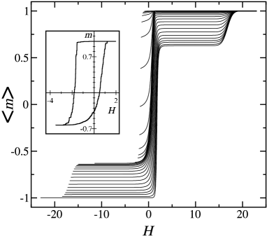
Figure 1: A set of FORCS for the EE-RFIM. They correspond to averages over 1000 realizations with $\sigma$ = 1.0 and $f$=0.05. The inset shows an example of a hysteresis loop with EB obtained with the same parameters, reversing the field at $H=-4$

an example of a hysteresis loop exhibiting EB. The reason behind this EB property is that such loops do, in fact, correspond to partial loops. The symmetric loop is obtained after applying very negative ($\propto J_{E}$) external fields.

In this short paper we present an analysis of the First-Order Reversal Curves (FORC) of the EE-RFIM corresponding to the case $J_{E}=20$ and $f=0.05$ obtained from the simulation of a $L=50$ lattice. Other interesting properties of this model have been published elsewhere [3].

A set of FORC is shown in Fig. 1. In order to analyze the structure of this set of FORC curves, we compute the so called FORC diagram. This is obtained by calculating the mixed second derivative of the magentization $m$ at field $H_{b}$ on a FORC obtained with reversal point $H_{a}$ [4]:

$$\rho(H_{a},H_{b})=-\frac{\partial^{2}m(H_{a},H_{b})}{\partial H_{a}\partial H_{b}}$$ (2)

The values of $\rho$ are usually represented on a diagram which is obtained after rotating the co-ordinates according to $H_{c}=(H_{b}-H_{a})/2$ and $H_{u}=(H_{a}+H_{b})/2$. The new co-ordinates allow a direct comparison with the Preisach distributions [5]. Fig. 2 shows the central part of the FORC diagram corresponding to the standard RFIM (a) and to the EE-RFIM (b). The comparison reveals that the EB property is reflected by a displacement of the central peak to the bottom. The vertical width of this peak increases when the width $\sigma$ of the random field distribution also becomes larger. The shift to the bottom is also greater for increasing $f$. Furthermore, other interesting features appear on the FORC diagram. These can be observed on the wider map in Fig. 3. The two main characteristics are the occurrence of an oscillation in the $H_{u}<0$ region and a second peak in the region of large values of $H_{c}$ ($\sim 17$).

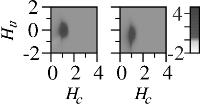
Figure 2: Averaged FORC diagram of the RFIM (a) and the EE-RFIM (b) corresponding to $\sigma=2$. The scale on the right indicates the values of $\rho$ corresponding to different shades of grey.

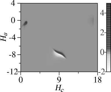
Figure 3: FORC diagram corresponding to the set of curves in Fig. 1.

An interesting point to make is that the oscillation includes a region of negative values of $\rho$. Neither this negative region nor the asymmetry of Fig. 3 can be interpreted within the framework of the Preisach model for which $\rho$ is assumed to be a probability density which should always be positive and symmetric about the $H_{u}=0$ axis. The negatives values of $\rho$ are associated with the fact that the slope of the $m(H)$ curves at $-1<H<0$ increases when $H_{a}$ becomes larger. It will be very interesting to analyze whether such singular features occur for experimental systems with EB. This will reveal the non-Preisach nature of such bilayered systems. We acknowledge fruitful comments from J.Nogués and H.G.Katzgraber.

References

- [1] J.P.Sethna, K.Dahmen, S.Kartha, J.A.Krumhansl, B.W.Roberts and J.D.Shore, Phys. Rev. Lett. 70 (1993) 3347.
- [2] J.Nogués and I.K.Schuller, J. Magn. Magn. Mater. 192, 203 (1999).
- [3] X.Illa, E.Vives and A.Planes, Phys. Rev. B 66 (2002) 224422.
- [4] C.R.Pike, A.P.Roberts and K.L.Verosub, Journ. Appl. Phys. 85 (1999) 6660; H.G.Katzgraber et al., Phys. Rev. Lett. 89 (2002) 277202.
- [5] G.Bertotti, Hysteresis in Magnetism, Academic Press, San Diego, 1998.