Statistical properties of pinning fields in the 3d-Gaussian RFIM

Abstract

We have defined pinning fields as those random fields that keep some of the magnetic moments unreversed in the region of negative external applied field during the demagnetizing process. An analysis of the statistical properties of such pinning fields is presented within the context of the Gaussian Random Field Ising Model (RFIM). We show that the average of the pinning fields exhibits a drastic increase close to the coercive field and that such an increase is discontinuous for low degrees of disorder. This behaviour can be described with standard finite size scaling (FSS) assumptions. Furthermore, we also show that the pinning fields corresponding to states close to coercivity exhibit strong statistical correlations.

,

1 Introduction

The magnetization reversal process in a ferromagnet is a complex dynamical process which is still not totally understood [1] . It is, nevertheless, very important for both fundamental and technological reasons. Different factors play a role in determining the metastable path that the system follows to reverse the magnetization from full positive saturation to full negative saturation when the external field is decreased. Among others, thermal fluctuations, long range dipolar forces, anisotropy and local forces due to disorder, compete together in order to decide the sequence of magnetic domains that transform.

A first simplification of the problem consist in neglecting the role of fluctuations and relaxation effects. This corresponds to the limiting case of “rate-independent” hysteresis. Magnetization reversal steps occur as almost instantaneous avalanches joining metastable states. Such avalanches are triggered when the external forces induced by the applied field are strong enough to overcome the internal energy barriers which are caused by exchange forces, long-range dipolar forces and forces created by disorder.

A prototypical model for the study of the influence of disorder in such an “athermal case” is the Gaussian RFIM. This model has been studied using two different approaches. On the one hand, a number of studies[2, 3] have focused on the analysis of a single magnetic interface. The numerical algorithms assume that only spins close to the interface can flip. On the other hand, studies including both nucleation events and interface motion have been performed by using synchronous relaxation dynamics [4, 5]. In both cases hysteresis appears as a consequence of the local fields that keep the magnetic moments unreversed (pinned) even at negative values of the applied external field. We will focus on the statistical analysis of such pinning fields in the case of RFIM with synchronous relaxation dynamics.

Our goal is to point out an essential difference between the two approaches. The quenched pinning fields originating from disorder exhibit very different statistical distributions in both cases. The distribution of pinning fields in an intermediate state is very different from the quenched disorder distribution corresponding to the initial saturated state (Gaussian) in lattice models that include nucleation and interface movement. This is due to the fact that in the initial stages of the demagnetization process the regions with low energy barriers have already been reverted. Close to coercivity, the remaining barriers are much higher due to the previous selection process. Such an effect does not occur for the models with an advancing single interface, for which the pinning fields in the unreversed regions always exhibit a statistical distribution which corresponds to the original quenched disorder distribution.

2 Model

The 3d-Gaussian RFIM at $T=0$ is defined on a cubic lattice of size $N=L^{3}$. On each lattice site a variable $S_{i}=\pm 1$ accounts for the magnetic degrees of freedom. The Hamiltonian is:

$$H=-\sum_{ij}S_{i}S_{j}-\sum_{i}S_{i}h_{i}-B\sum_{i}S_{i}$$ (1)

where the first term stands for the exchange interaction between nearest-neighbour spins $S_{i}$, the second term for the interaction with the quenched local random fields $h_{i}$ and the last term for the interaction with the driving field $B$. The $h_{i}$ are Gaussian distributed with zero mean and variance $\sigma^{2}$. Although this model enable long-range dipolar forces to be included, from a computational point of view the numerical solution becomes much harder. Since we are interested in the analysis of the pinning fields generated by disorder, we have neglected long-range terms.

The numerical simulations are performed using local relaxation dynamics [4]. The initial saturated state with all the spins $S_{i}=1$ corresponds to the equilibrium state with $B=+\infty$. The field $B$ is then decreased until a spin $S_{i}$ becomes locally unstable. At this point the external field is kept constant and the spin $S_{i}$ is flipped. This may cause an avalanche since some of its neigbouring spins may become unstable. All unstable spins are flipped synchronously, until the avalanche ends. The external field $B$ is then decreased again until a new avalanche starts.

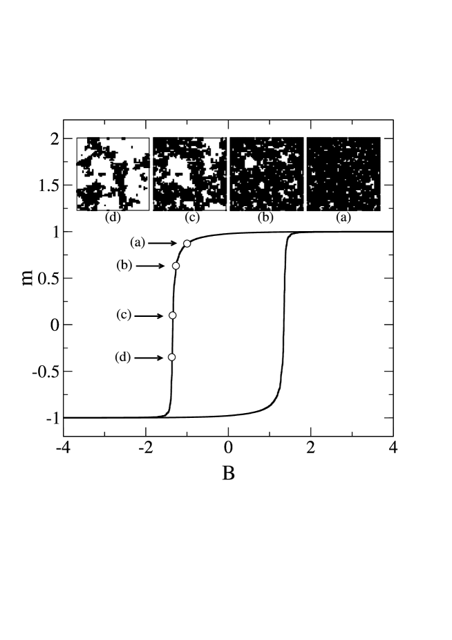
Figure 1: Example of a hysteresis loop corresponding to $\sigma=2.5$ and $L=60$. The insets show examples of typical spin configurations.

The hysteresis loop is obtained by measuring the magnetization $m=\sum_{i=1}^{N}S_{i}/N$ as a function of $B$. Fig. 1 shows an example and the corresponding configurations snapshots. As can be seen, nucleation and interface movement coexist during evolution. Due to the finite size of the simulated system, the loops consist of a sequence of discontinuous jumps or avalanches for each realization of the random fields $h_{i}$. As has been studied in previous works [6, 7], the characteristics of the loops depend on the amount of disorder $\sigma$ in the thermodynamic limit ($L\rightarrow\infty$): they are continuous for $\sigma>\sigma_{c}$, whereas they display a discontinuity (corresponding to a spanning avalanche) at the coercive field for $\sigma<\sigma_{c}$. This behaviour is associated with the existence of a “metastable” critical point on the $(B,\sigma)$ phase diagram located at $\sigma_{c}=2.21$ and $B_{c}=-1.425$. The behaviour close to this critical point can be described by a set of critical exponents. For instance, the correlation length diverges with an exponent $\nu\simeq 1.2$, the order parameter (the magnetization jump $\Delta m$) goes to zero with an exponent $\beta\simeq 0.024$ when $\sigma\rightarrow\sigma_{c}$ from below and, at $\sigma=\sigma_{c}$, the magnetization behaves as $m\sim|B-B_{c}|^{1/\delta}$ with $\delta\simeq 50$. Such critical exponents have been obtained by detailed FSS analysis[6] which has also revealed that the most convenient scaling variable that measures the distance to $\sigma_{c}$ is

$$u=\frac{\sigma-\sigma_{c}}{\sigma_{c}}+A\left(\frac{\sigma-\sigma_{c}}{\sigma_{c}}\right)^{2}$$

with $A=-0.2$. Furthermore, since we will be interested in the measurement of properties as a function of the external field $B$, we will need a second scaling variable to measure the distance to $B_{c}$. The first simpler choice is:

$$v=\frac{B-B_{coe}}{B_{coe}}$$ (2)

where $B_{coe}(\sigma,L)$ is the coercive field that tends to $B_{c}$ when $\sigma\rightarrow\sigma_{c}$ and $L\rightarrow\infty$.

3 Results

We define pinning fields $h_{i}^{+}$ as those quenched random fields $h_{i}$ for which $S_{i}=+1$ during the reversal process for a certain intermediate configuration. Although the set of pinning fields is simply a subset of the original quenched random fields, their statistical properties depend on the exact path followed until a certain configuration is reached. We have computed the average value of the pinning fields $\langle h_{i}^{+}\rangle$ and the histograms corresponding to their statistical distribution $f(h_{i}^{+})$ as a function of $B$ and $\sigma$ by simulating many realizations of disorder. Moreover we have measured pair correlations as $C(h_{i}^{+},h_{j}^{+})=L^{3}\left(\langle h_{i}^{+}h_{j}^{+}\rangle-\langle h_{i}^{+}\rangle^{2}\right)$.

Fig. 2 shows the evolution of the distribution of pinning fields along the decreasing branch of a hystereis loop corresponding to $\sigma=2.14<\sigma_{c}$. This distribution can be understood as the distribution of barriers created by the quenched disorder that keeps the spins in the metastable state. Although initially the distribution of pinning fields is similar to the original Gaussian distribution, as the magnetization decreases, $f(h_{i}^{+})$ starts to develop a non-trivial structure. In general the distribution tends to shift to the right, towards the region of large pinning fields, but it also develops a number of peaks associated with the seven possible local magnetization environments.

Figs. 3 and 4 display the evolution of $\langle h_{i}^{+}\rangle$ and $C(h_{i}^{+},h_{j}^{+})$ as a function of the external field $B$ for two different values of $\sigma$ corresponding to two cases: above and below $\sigma_{c}$. It is interesting to point out that the correlation is not zero in the two cases and displays a peak close to the coercive field. Note that this means that the distributions $f(h_{i}^{+})$ are only projections of complex multivariate distributions. Additionally, $\langle h_{i}^{+}\rangle$ displays a discontinuity for $\sigma<\sigma_{c}$. The behaviour of $\langle h_{i}^{+}\rangle$ is, therefore, similar to the behaviour of an order parameter around a critical point.

Quantitative analysis of such data requires a convenient FSS analysis to be carried out. The two analyzed properties $\langle h_{i}^{+}\rangle$ and $C(h_{i}^{+},h_{j}^{+})$ are functions of the external field $B$, the amount of disorder $\sigma$ and the system size $L$. The FSS ansatz allows to the singular (critical) contributions of these two properties to be expressed as a function of the invariants $x=uL^{1/\nu}$ and $y=vL^{\beta\delta/\nu}$ :

$$\langle h_{i}^{+}\rangle=L^{-\theta}{\tilde{h}}\left(uL^{1/\nu},vL^{\beta\delta/\nu}\right)$$ (3)

$$C(h_{i}^{+},h_{j}^{+})=L^{3-\rho}{\tilde{C}}\left(uL^{1/\nu},vL^{\beta\delta/\nu}\right)$$ (4)

The exponents $\theta$ and $3-\rho$ characterize how $\langle h_{i}^{+}\rangle$ decreases and how the correlation $C$ diverges. Figures 5 and 6 show the scaling functions ${\tilde{h}}$ and ${\tilde{C}}$. The good quality of the collapses of data corresponding to different system sizes, confirms the scaling assumptions. The exponents that allow the best collapses are $\theta\simeq 0.41$ and $3-\rho\simeq 1.80$. Moreover, the behaviour of the scaling functions allows prediction of how the average pinning field and the correlations behave in the thermodynamic limit. Since $\tilde{h}$ behaves as $y^{\theta\nu/\beta\delta}$ for $v<0$ (as indicated by the discontinuous line) , $\langle h_{i}^{+}\rangle$ is finite for $B<B_{c}$. The scaling behaviour for $v>0$ is not so good since there are non-scaling contributions due to the existence of non-spanning avalanches for all values of $\sigma$ [6]. As regards correlations, the scaling functions display a peak profile which indicates that, besides non-scaling contributions, the correlation $C(h_{i}^{+},h_{j}^{+})$ will diverge at $B=B_{c}$ and $\sigma=\sigma_{c}$ in the thermodynamic limit.

4 Conclusions

Pinning fields are responsible for the energy barriers that keep the spins in the metastable state within the context of the 3d RFIM at $T=0$. The statistical distribution of pinning fields during the reversal magnetization process has been studied. Initially, when the system is saturated, the pinning fields are trivially distributed according to the nominal Gaussian distribution of random fields. As the demagnetizing process advances and domains of negative spins are created, the pinning fields display a complex distribution. Their mean value increases monotonously for decreasing $B$. For $\sigma>\sigma_{c}$ this increase is continuous but for $\sigma<\sigma_{c}$ the average pinning field displays a discontinuity at coercivity. Moreover we have shown that close to coercivity the pinning fields exhibit strong statistical correlations. We finally remark that such a complex behaviour of the distribution of pinning fields is not taken into account in the studies that focus on the analysis of an advancing single magnetic interface.

We acknowledge fruitful discussions with F.J.Pérez-Reche. This work has received financial support from CICyT (Project No MAT2001-3251) and CIRIT (Project 2001SGR00066). X.I. aknowledges financial support from DGI-MCyT (Spain).

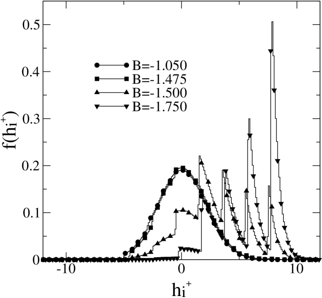
Figure 2: Examples of distributions $f(h_{i}^{+})$ corresponding to $L=60$, $\sigma=2.14$ and different values of the external field as indicated. Data corresponds to averages over $1000$ realizations of disorder.

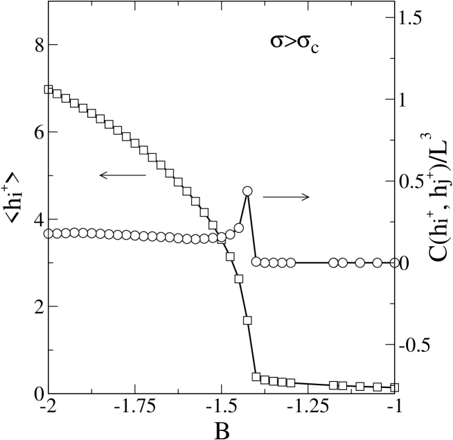
Figure 3: Example of the evolution of $\langle h_{i}^{+}\rangle$ and $C(h_{i}^{+},h_{j}^{+})$ as a function of the external field for a system with $L=60$ and $\sigma=2.28$. Data correspond to averages over 1000 realizations of disorder.

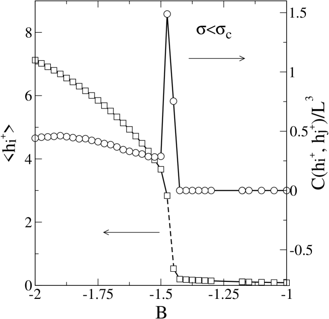
Figure 4: Example of the evolution of $\langle h_{i}^{+}\rangle$ and $C(h_{i}^{+},h_{j}^{+})$ as a function of the external field for a system with $L=60$ and $\sigma=2.14$. Data correspond to averages over 1000 realizations of disorder.

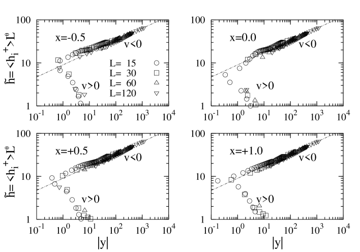
Figure 5: FSS analysis of the average pinning field $\langle h_{i}^{+}\rangle$. The figures show, on log-log scales, the scaling function $\tilde{h}$ in front of $y=vL^{\beta\delta/\nu}$ for 4 different values of $x=uL^{1/\nu}$ as indicated on each graph. Data correspond to the overlap of sizes $L=15,30,60,120$ (as indicated by the legend) and averages over many realizations of disorder ranging from $10^{6}$ to $10^{3}$.

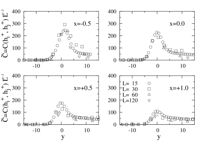
Figure 6: FSS analysis of the correlation between pinning fields $C(h_{i}^{+},h_{j}^{+})$. Details are the same as in Fig. 5.

References

- [1] G. Bertotti, Hysteresis in Magnetism, Academic Press (San Diego, )
- [2] B.Koiller and M.O.Robbins, Phys. Rev. B 62, 5771 (2000).
- [3] L.Roters, A.Hucht, S.Lübeck, U.Nowak and K.D.Usadel, Phys. Rev. E 60, 5202 (1999), and references therein
- [4] J.P. Sethna, K. Dahmen, S. Kartha, J.A. Krumhansl, B.W. Roberts, and J.D. Shore, Phys. Rev. Lett. 70 (1993) 3347
- [5] J.P. Sethna, K.A. Dahmen, and C.R. Myers, Nature 410 (2001) 242
- [6] F.J. Pérez-Reche and E. Vives, Phys. Rev. B 67 (2003) 134421, and references therein.
- [7] O.Perkovic, K.A.Dahmen and J.P.Sethna, Phys. Rev. B 59 (1999) 6106, and references therein.