Dynamics of sliding drops on superhydrophobic surfaces

Abstract

We use a free energy lattice Boltzmann approach to investigate numerically the dynamics of drops moving across superhydrophobic surfaces. The surfaces comprise a regular array of posts small compared to the drop size. For drops suspended on the posts the velocity increases as the number of posts decreases. We show that this is because the velocity is primarily determined by the contact angle which, in turn, depends on the area covered by posts. Collapsed drops, which fill the interstices between the posts, behave in a very different way. The posts now impede the drop behaviour and the velocity falls as their density increases.

1 Introduction

The aim of this letter is to explore numerically how micron-scale drops move on superhydrophobic surfaces. If surfaces with contact angles greater than $90^{o}$ are patterned with posts small compared to the drop dimensions the equilibrium contact angle is increased and can reach values close to $180^{o}$. Such superhydrophobic surfaces are found in nature: for example the leaves of several plants, such as the lotus are covered in tiny bumps which may have evolved to aid the run-off of rain water. Recent microfabrication techniques have allowed superhydrophobic patterning to be mimicked and carefully controlled experiments on the behaviour of drops on superhydrophobic substrates are increasingly becoming feasible[1].

Drops on superhydrophobic surfaces can be in two states. Suspended drops lie on top of the posts with air pockets beneath them whereas collapsed drops fill the interstices between the posts. A suspended drop has a higher contact angle than the equivalent collapsed drop which in turn has a higher contact angle than a drop on a flat surface made of the same material. Several authors have shown that the equilibrium properties of the drops follow from thermodynamic arguments based on free energy minimisation [2, 3, 4, 5]. Both the suspended and collapsed states can provide the global minimum of the free energy, with the phase boundary between them depending on the surface tension, the contact angle on the flat surface and the post geometries [6, 7]. The suspended drop may often exist as a metastable state as it has to cross a free energy barrier to fill the grooves [3, 8].

There is, however, no similar understanding of the way drops move across superhydrophobic surfaces. Several authors [9, 10, 11] have considered contact angle hysteresis in the context of whether a drop is pinned or moves as a surface is tilted. The consensus of both theoretical and experimental work is that a suspended drop on a superhydrophobic surface starts to move much more easily than the equivalent drop on a smooth surface.

Only a few results have been published about the steady-state velocities of moving drops. Gogte et al. [12] have shown that the drag on a hydrofoil decreases by $\sim 10\%$ if it is covered by a superhydrophobic coating. Ou et al. [13] have shown experimentally that a drag reduction $\sim 40\%$ can be obtained for drops on surfaces with micron-scale posts. Cottin-Bizonne et al. [6] have used molecular dynamics simulations to explore the behaviour of a fluid moving across a superhydrophobic surface comprising nanometre posts. They find that the slip is enhanced by a factor $\sim 2.5$ when the fluid does not fill the space between the posts and reduced by a factor $\sim 10$ when it does, as compared to a flat surface of the same (hydrophobic) material.

In this letter we explore movement across a superhydrophobic surface by using a lattice Boltzmann approach to solve the equations of motion of a drop pushed gently by a constant force. This approach has been shown to agree well with experiments for spreading and moving drops on chemically striped surfaces [14, 15]. Here we consider both suspended and collapsed drops on superhydrophobic surfaces and investigate how the drop velocity depends on the post spacing. We find that the velocity of suspended drops is essentially determined by the effective contact angle and increases as the number of posts decreases. Collapsed drops, however, behave in a very different way. The posts now impede the drop behaviour and for large post densities the flow pushes the drop back to a suspended position on top of the posts.

2 The model

We consider a liquid-gas system of density $n({\mathbf{r}})$ and volume $V$. The surface is denoted by $S$. The equilibrium properties of the drop are described by the Ginzburg-Landau free energy

$$\Psi=\int_{V}\left(\psi_{b}(n)+\frac{\kappa}{2}\left(\partial_{\alpha}n\right)^{2}\right)dV+\int_{S}\psi_{c}(n)\;dS$$ (1)

where Einstein notation is understood for the Cartesian label $\alpha$. $\psi_{b}(n)$ is the free energy in the bulk. For convenience we choose a double well form.

The derivative term in equation (1) models the free energy associated with density gradients at an interface. $\kappa$ is related to the surface tension. $\psi_{c}(n_{s})=-\phi_{1}n_{s}$, where $n_{s}$ denotes the density at the surface, is the Cahn surface free energy [17] which controls the wetting properties of the fluid. In particular $\phi_{1}$ can be used to tune the contact angle.

The dynamics of the drop is described by the Navier-Stokes equations for a non-ideal gas

$$\partial_{t}(nu_{\alpha})+\partial_{\beta}(nu_{\alpha}u_{\beta}) = -\partial_{\beta}P_{\alpha\beta}+\nu\partial_{\beta}\big{[}n(\partial_{\beta}u_{\alpha}+\partial_{\alpha}u_{\beta}+\delta_{\alpha\beta}\partial_{\gamma}u_{\gamma})\big{]}+nF_{\alpha},$$ (2)

$$\partial_{t}n+\partial_{\alpha}(nu_{\alpha}) = 0$$ (3)

where $\mathbf{u}({\mathbf{r}})$ is the fluid velocity, $\nu$ the kinematic viscosity and $n\mathbf{F}$ a body force per unit volume. In what follows, we will refer the second term on the right hand side of the first equation as the viscous term. The pressure tensor $P_{\alpha\beta}$ is calculated from the free energy [16].

We use a lattice Boltzmann algorithm that solve the equations of motion by following the evolution of particle distribution functions. This corresponds to a discretisation of a simplified Boltzmann equation. Details can be found in [8].

3 Results

We consider a drop of radius 30 moving on a domain of size $L_{x}\times L_{y}\times L_{z}=80\times 80\times 80$ lattice sites. Periodic boundary conditions are imposed along $x$ and $y$. The surface at $z=L_{z}-1$ is flat and that at $z=0$ is patterned by posts in a square array with height, spacing and width denoted by $h$, $d$ and $w$ respectively. Unless otherwise specified $h=5$. A contact angle $\theta_{0}=110^{o}$ is set on every substrate site by choosing a suitable value of the surface field $\phi_{1}$. In equilibrium the drop forms a spherical cap with an enhanced contact angle. For example, if $d=8$ and $w=4$ the contact angle is $156^{o}$ for a drop resting on the posts and $130^{o}$ for a drop collapsed between the posts [8].

We impose a Poiseuille flow by considering a constant body force $nF_{x}$ per unit volume parallel to the surface corresponding to a Bond number $Bo=V^{2/3}nF_{x}/\gamma=1.42$ where $\gamma$ is the surface tension and $V$ the drop volume. Fig. 1(a) shows the time average capillary number $Ca=\nu Un_{l}\gamma^{-1}$ of the suspended drop as the width of the posts and the distance between the posts are varied. $U$ is the velocity of the drop and $n_{l}$ the liquid density. The $w/d=0$ result corresponds to a drop moving on a cushion of air (of height $5$), and the $w/d=1$ value to a drop moving on a flat surface of contact angle $110^{o}$. It is striking how the data collapses onto a single curve if it is plotted as a function of the ratio $w/d$. We also measured the velocity of drops moving on a ridged surface, considering both a drop moving parallel and perpendicular to the ridges. This data also collapses onto the same curve if plotted as a function of $(w^{*}/d^{*})^{1/2}$, where $w^{*}$ is the width of the ridges and $d^{*}$ the spacing between them.

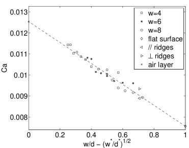
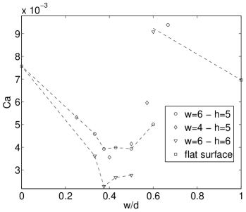
(a)		(b)

Figure 1: Steady state capillary number of (a) suspended (b) collapsed drops. The height, spacing and width of the posts are denoted by $h=5$, $d$ and $w$ respectively (in simulation units, compared to the drop radius $R=30$). A contact angle $\theta_{0}=110^{o}$ is set on every substrate site. We impose a Poiseuille flow with $Bo=1.42$. The data is plotted as a function of $(w/d)$ for surfaces with posts and $(w^{*}/d^{*})^{1/2}$ when ridged surfaces are considered. A vertical velocity is imposed on collapsed drops for them to cross the suspended to collapsed free energy barrier. The variation in the velocity of the drop because of its position relative to the posts is less that $1\%$ in (a) and less than $5\%$ in (b).

Fig. 1(b) compares the behaviour of a collapsed drop driven by the same force. The dependence of the velocity on the length ratio $w/d$ is now very different.

From the results of fig. 1 we can formulate the questions that need to be answered to understand the way in which the drops move over the posts. Firstly why is the velocity controlled by the ratio $w/d$ for the drops suspended on the posts? Secondly why is the behaviour of the collapsed drop more complicated with seemingly two different regimes as $w/d$ increases from zero to unity? To answer these questions it is helpful to first consider in some detail the behaviour of a drop moving on a flat surface.

We therefore consider a system of size $L_{x}\times L_{y}\times L_{z}=80\times 80\times 40$ with no-slip walls at $z=0$ and $z=L_{z}-1$ and periodic boundary conditions along $x$ and $y$. A liquid droplet is placed on the surface at $z=0$ and forms a spherical cap of contact angle $\theta_{0}$.

We impose a Poiseuille flow by setting a body force $nF_{x}$ per unit volume along $x$. The droplet becomes slightly elongated along the flow direction and increases the front and decreases the back contact angle. For example, the steady state of a drop of radius $R=18$ with $\theta_{0}=70^{o}$ pushed by a force corresponding to $Bo=6.4$ is depicted in fig. 2. The front and back contact angles become $\theta_{f}=73.2^{o}$ and $\theta_{b}=67.1^{o}$. This occurs because, in order that the drop can move, the contact line has to slide along the surface, in a way that does not violate the non-slip boundary conditions on the velocity field. This is mediated by the advancing and receding contact angles deviating from their equilibrium values so that the interface does not have the correct radius of curvature. Terms in the pressure tensor act to restore the equilibrium curvature.

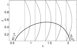
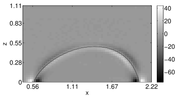
(a)		(b)

Figure 2: Steady state of a sliding droplet with $\theta_{0}=70^{o}$ in a Poiseuille flow with $Bo=6.4$. The advancing and receding contact angles are $73.2^{o}$ and $67.1^{o}$. (a) Cut along $y=L_{y}/2$. The thick line is the interface where $n({\mathbf{r}})=n_{c}$. The thin solid lines are velocity profiles when the drop is in place. Dashed lines are velocity profiles with no drop. (b) $x$-component of the viscous term in the Navier-Stokes equation (dimensionless units, scaled by $V^{(2/3)}/\gamma$) across the same cross section. Length is dimensionless scaled by the drop diameter $D$.

Our first aim is to understand what determines the velocity of the drop. Fig. 2(a) shows the flow profile with and without the drop in place. There is very little change due to the presence of the drop, $<10\%$ in all the simulations reported here. (Considering different viscosities for drop and vapor leads to the same conclusion.) To tie in with this we would expect the extra dissipation due to the presence of the drop to be relatively small. The magnitude of $x$-component of the viscous term in different regions of the drop is shown in fig. 2(b). The dissipation is increased near the interface and, particularly, near the contact line. However this increase represents only a few percent of the total viscous dissipation; the rest being due to the Poiseuille flow in the bulk.

Thus the drop is effectively convected along by the flow field and its velocity is determined by its position within this flow. If the drop radius or the contact angle are larger, the drop centre of mass lies at a higher $z$ position within the flow and the drop therefore moves faster.

This is illustrated in fig. 3 where we compare the velocity of the drop and the speed of the flow at the position of its centre of mass for different drop radii, equilibrium contact angles, and imposed forces. There is close qualitative and reasonable quantitative ($\sim 10\%$) agreement. An exact match is not to be expected because of the enhanced dissipation around the interface.

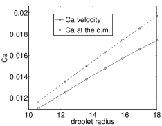
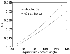
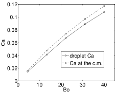
(a)	(b)	(c)

Figure 3: Variation of drop capillary number with (a) radius $R$ (in simulation units) for $Bo=6.41$ and $\theta_{0}=70^{o}$; (b) contact angle for $R=15$ and $Bo=6.41$; (c) driving force for $R=15$ and $\theta_{0}=70^{o}$.

We are now in a position to explain the results in fig. 1(a), in particular that the velocity of the drop depends on $w/d$, the ratio of the post width $w$ and the post spacing $d$. This follows because the velocity of the drop is primarily determined by its position within the flow field which depends on the apparent contact angle. This, in turn, is determined, through Cassie’s law by $w/d$, for a given value of the flat surface contact angle.

This can be made more quantitative if we approximate the shape of the suspended drop as a spherical cap. Cassie’s law relating the flat surface contact angle $\theta_{0}$ to the observed contact angle on the superhydrophobic substrate $\theta$ is

$$\cos\theta=(w/d)^{2}(\cos\theta_{0}+1)-1.$$ (4)

The position of the centre of mass of the drop is

$$\bar{z}=\bar{R}\left\{\frac{3-8\cos\theta+6\cos^{2}\theta-\cos^{4}\theta}{8-12\cos\theta+4\cos^{3}\theta}\right\}\quad\textrm{with}\quad\bar{R}=R\left\{\frac{4}{2-3\cos\theta+\cos^{3}\theta}\right\}^{1/3}$$ (5)

where $\bar{R}$ is the radius of the spherical cap. For Poiseuille flow the dimensionless velocity is

$$v_{x}^{*}=\frac{4Bo}{(4/3\pi)^{2/3}}\left(\bar{z}-\frac{\bar{z}^{2}}{D_{c}}\right)$$ (6)

where $D_{c}$ is the diameter of the channel and $\nu=0.1$ is the kinematic viscosity.

Table 1 compares the numerical results to equation (6) with $D_{c}=L_{z}-h$. As before the formula agrees qualitatively with the simulations and predicts a velocity $\sim 10\%$ higher than that measured. For smaller values of $w/d$ the numerical and analytic results are closer, but this is because the effective width of the channel decreases as the number of posts increase.

$w/d$	simulated $Ca$ (from fig. 1)	estimated velocity, $v_{x}^{*}$ (from equation (6))
1	$0.0076$	$0.0089$
0.73	$0.0089$	$0.0102$
0.6	$0.0096$	$0.0107$
0.4	$0.0104$	$0.0113$
0.25	$0.0114$	$0.0116$

Table 1: Comparison of simulated and estimated velocity for a drop moving across a superhydrophobic surface.

Fig. 1(b) shows that a different mechanism is in play for collapsed drops. To understand this we consider flow over a $4\times 4$ square post of height $5$ centered within a domain of size $L_{x}\times L_{y}\times L_{z}=50\times 40\times 40$ lattice sites. The contact angles on the post and on the surface are identical, $\theta_{0}=110^{o}$. No-slip velocity boundary condition are imposed on every substrate site. A droplet of radius $R=15$ is equilibrated away from the post. The drop is convected by a Poiseuille flow with $Bo=4.5$ until it eventually meets the post. Dissipation due to friction occurs at the top of the post as it distorts the flow field as shown in fig. 4(a).

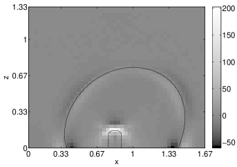
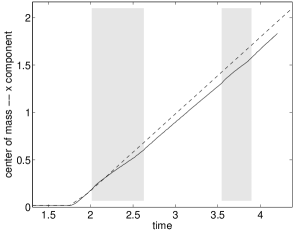
(a)		(b)

Figure 4: (a) $x$-component of the viscous term in the Navier-Stokes equation (in dimensionless unit, scaled by $V^{(2/3)}/\gamma$) for a drop moving across a surface decorated with a single post. Cross section at $y=L_{y}/2$. (b) Comparison of the variation of the position of the centre of mass with time of two drops. Dashed line: drop moving across a flat surface. Full line: drop moving across a surface decorated by a post. Both length and time are dimensionless scaled by the drop diameter $D$ and $\nu nD/\gamma$ respectively. The grey areas between $t=2$ and $t=2.6$ and between $t=3.5$ and $t=3.9$ correspond to the advancing and to the receding contact lines being on the post respectively. $\theta_{0}=110^{o}$ on every surface site.

Fig. 4(b) compares the velocity of two drops, one (F) moving on a flat surface and the other (P) over a post. The velocities cease to be identical as soon as the drop meets the post. Because of the distortion of the flow field the velocity of P is lower than that of F. The velocities become identical again as soon as the drop leaves the post. The velocity difference decreases as the height of the posts is decreased.

With this information we return to fig. 1(b). Increasing $w/d$ from $0$ corresponds to inserting posts into the drop path. As shown above this leads to increased dissipation as the posts distort the flow field. Hence the velocity drops, the decrease being greater for the higher posts.

For $w/d$ above $\sim 0.7$, the velocity jumps to a higher value and then decreases as more posts are inserted. Here the velocities are identical to those measured for the suspended drop (see fig. 1(a)). This is because the force drives a transition from the collapsed to the suspended state when posts cover a large fraction of the surface. The complicated behaviour for $w/d\sim 0.5$ occurs because parts of the drop are collapsed and parts suspended.

4 Conclusion

We have solved the hydrodynamic equations of motion for drops sliding over superhydrophobic surfaces. For drops suspended on the surfaces there is an increase in velocity of about $50\%$ as the number of posts is decreased to zero. We show that the main contribution to this effect is from the position of the drop in the Poiseuille flow field. As the number of posts is decreased the contact angle increases and hence the drop lies, on average, further from the surface. Thus it is subjected to a higher velocity field and moves more quickly.

For collapsed drops the situation is very different. Here, as posts are introduced, they impede the drop and its velocity falls. For a large number of posts, as the drop is pushed, it prefers to revert to the suspended state.

These results are consistent with the few experiments in the literature [12, 13]. However the model we solve does include approximations to make it numerically tractable and it is important to be aware of these. In particular interfaces tend to move too easily, because, as with all mesoscale two-phase fluid simulations, simulated interface widths are too wide. The effect of this is that, given a set of input physical parameters, the simulation drop will move more quickly than a real drop. This can be accounted for by a rescaling of time by, for example, matching the capillary number at which the moving drop develops a corner in its trailing edge to experiment [18]. Moreover it is necessary to choose boundary condition for the model. We have taken a non-slip condition on the velocity on every surface site: although there is evidence for increased local slip on hydrophobic surfaces this is still on the nano metre level and so would not show up on the scale of these simulations.

The drops we consider are in the sliding, rather than the rolling regime. Most experiments to date have been on highly viscous drops which roll [19], but it is likely that there will soon be experiments on drops with lower viscosity which will allow interesting comparisons to the simulations reported here.

5 Acknowledgment

AD acknowledges the support of the EC IMAGE-IN project GR1D-CT-2002-00663. We thank H. Kusumaatmaja for useful comments on the draft.

References

- [1] \NameD. Quéré \ReviewRep. Prog. Phys. \Vol68 \Year2005 \Page2495
- [2] \NameC. Ishino, K. Okumura, and D. Quéré \ReviewEurophys. Lett. \Vol68 \Year2004 \Page419
- [3] \NameN. Patankar \ReviewLangmuir \Vol20 \Year2004 \Page7097
- [4] \NameA. Marmur \ReviewLangmuir \Vol19 \Year2003 \Page8343
- [5] \NameP. Swain and R. Lipowsky \ReviewLangmuir \Vol14 \Page6772 \Year1998
- [6] \NameC. Cottin-Bizonne et al.\ReviewNature Materials \Vol2 \Year2003 \Page237
- [7] \NameC. Journet et al. \ReviewEurophys. Lett. \Vol71 \Year2005 \Page104
- [8] \NameA. Dupuis and J. Yeomans \ReviewLangmuir \Vol21 \Year2005 \Page2624
- [9] \NameB. Krasovitski and A. Marmur \ReviewLangmuir \Vol21 \Year2005 \Page3881
- [10] \NameD. Öner and T. McCarthy \ReviewLangmuir \Vol16 \Year2000 \Page7777
- [11] \NameG. McHale, N. Shirtcliffe, and M. Newton \ReviewLangmuir \Vol20 \Year2004 \Page10146
- [12] \NameS. Gogte et al. \ReviewPhys. Fluids \Vol17 \Year2005 \Page051701
- [13] \NameJ. Ou, B. Perot, and J. Rothstein \ReviewPhys. Fluids \Vol16 \Year2004 \Page4635
- [14] \NameA. Dupuis and J.M. Yeomans \ReviewFut. Gen. Comp. Syst. \Vol20 \Page993 \Year2004
- [15] \NameH. Kusumaatmaja et al. \ReviewEurophys. Lett. \Vol73 \Page740 \Year2006
- [16] \NameM.R. Swift et al. \ReviewPhys. Rev. E \Vol54 \Page5051 \Year1996
- [17] \NameJ. Cahn \ReviewJ. Chem. Phys. \Vol66 \Year1977 \Page3667
- [18] \NameT. Podgorski, J.-M. Flesselles, and L. Limat \ReviewPhys. Rev. Lett. \Vol87 \Year2001 \Page036102
- [19] \NameD. Richard and D. Quéré \ReviewEurophys. Lett. \Vol48 \Year1999 \Page286