Single-site approximation
for reaction-diffusion processes
xxx

Abstract

We consider the branching and annihilating random walk $A\to 2A$ and $2A\to 0$ with reaction rates $\sigma$ and $\lambda$, respectively, and hopping rate $D$, and study the phase diagram in the $(\lambda/D,\sigma/D)$ plane. According to standard mean-field theory, this system is in an active state for all $\sigma/D>0$, and perturbative renormalization suggests that this mean-field result is valid for $d>2$; however, nonperturbative renormalization predicts that for all $d$ there is a phase transition line to an absorbing state in the $(\lambda/D,\sigma/D)$ plane. We show here that a simple single-site approximation reproduces with minimal effort the nonperturbative phase diagram both qualitatively and quantitatively for all dimensions $d>2$. We expect the approach to be useful for other reaction-diffusion processes involving absorbing state transitions.

Keywords: reaction-diffusion problems, branching processes.

LPT – ORSAY 06/04                                                 
^∗Laboratoire associé au Centre National de la Recherche Scientifique - UMR 8627

1 Introduction

Branching and annihilating random walks (BARW [1]) have been the focus of much attention [2, 3, 4, 5, 6, 7], as they are among the simplest models of nonequilibrium critical phenomena observed in physics and other sciences (for reviews see, e.g., [8, 9, 10]). They are generic reaction-diffusion processes in which particles of some species $A$ move stochastically on an arbitrary $d$-dimensional lattice and are subject to the creation and annihilation reactions $A\xrightarrow{\sigma_{m}}(m+1)A$ and $kA\xrightarrow{\lambda_{k}}0$. The nonequilibrium phase transitions of these models are known to belong to two distinct universality classes, depending on the parity of $m$ and $k$: the “Parity Conserving” class (for $m$ and $k$ even) and the “Directed Percolation” class (for $m$ odd) [5, 8]. We are interested here in BARW belonging to the Directed Percolation class, which are generally denoted “odd-BARW”.

The simplest odd-BARW, which in this work we will call for short the “OBA model” (odd branching and annihilating walks), is defined by

$$\mbox{{OBA model}}\qquad\left\{\begin{array}[]{ll}A\xrightarrow{\sigma}2A\\[8.53581pt] 2A\xrightarrow{\lambda}0\\[8.53581pt] A\emptyset\xrightarrow{D}\emptyset A\end{array}\right.$$ (1.1)

where $\sigma$ and $\lambda$ are on-site creation and annihilation rates, respectively, and $D$ is a hopping rate between adjacent sites. If the lattice has coordination number $c$, this means that a particle will leave its lattice site at a rate $cD$. Since it captures the essential critical properties of its entire class [5], our focus will be specifically on the OBA model. Although it is well-established that the OBA model is in the Directed Percolation universality class [5], it has appeared much harder to determine its phase diagram, and this is the subject of this paper.

In standard mean-field (MF) theory [8, 5] the OBA model is described by the rate equation

$$\frac{\partial\rho}{\partial t}=D\Delta\rho+\sigma\rho-\lambda\rho^{2},$$ (1.2)

where $\rho(r,t)\geq 0$ is the particle density. For all branching ratios $\sigma\geq 0$ Eq. (1.2) has two spatially uniform stationary solutions, the “absorbing state” $\rho_{0}=0$ and the “active state” $\rho_{*}=\sigma/\lambda$. For $\sigma>0$ the active state is stable and is reached exponentially fast in time from any initial state with $\rho>0$. For $\sigma=0$ the OBA model coincides with the pure pair annihilation process (PA) and corresponds to a critical point in parameter space at which the absorbing state is reached according to the power law decay $\rho(r,t)\sim t^{-1}$.

On a lattice in finite dimension $d$ the question of the stationary states of (1.1) is much more difficult to answer. For $\sigma=0$, i.e. for the PA, perturbative renormalization group analysis has shown [11, 5] that below the critical dimension $d_{c}=2$ the decay to the absorbing state slows down due to depletion zones (anticorrelations) in the spatial density distribution and follows the power law $\rho(r,t)\sim t^{-d/2}$.

Early simulations of the OBA model [3, 4] showed that for $d=1$ and $d=2$ absorbing states exist even in an interval of branching ratios $\sigma>0$, in contradistinction to MF theory. This indicates, therefore, that low-dimensional fluctuations qualitatively change the “phase diagram” of this system in the $(\lambda,\sigma)$ plane.

In a seminal paper, Cardy and Täuber [5] formulated a field theory for general BARW, which they analyzed by perturbative renormalization group techniques. For the OBA model they concluded that in dimension $d\leq 2$ a minimum branching ratio $\sigma_{\rm c}$ is needed in order for the system to be able to sustain an active state. For small $\lambda$ the critical value $\sigma_{\rm c}$ behaves as

$$\sigma_{\rm c}\simeq D\Big{(}\frac{\lambda}{2D\pi\epsilon}\Big{)}^{2/\epsilon},\qquad\lambda\to 0,\qquad d=2-\epsilon.$$ (1.3)

The analysis by Cardy and Täuber is valid for small $\lambda$ and appears to break down for $d>2$ [5]. However, since $\lambda$ becomes irrelevant above two dimensions and since from the PA analysis one can assume that fluctuations are also small for $d>2$ in the OBA model when $\sigma$ is small, Cardy and Täuber argue that MF theory should be restored for $d>2$, that is, the system should be active for all $\sigma>0$ [5].

This picture was modified by an analysis due to Canet et al. [6, 7], who employed nonperturbative renormalization group (NPRG) techniques. They demonstrated that in all finite dimensions $d>2$ there is a threshold $\lambda_{\rm c}$ such that

i (i) for $\lambda<\lambda_{\rm c}$ the MF result of an active state for all $\sigma>0$ remains true, but

(ii) for $\lambda>\lambda_{\rm c}$ there is an active state only when $\sigma>\sigma_{\rm c}(\lambda)$.

Hence according to the work of Ref. [6, 7] standard MF theory fails dramatically for this system.

Following this failure, the OBA model has been re-investigated [13] by means of an alternative MF type approximation, namely the “cluster MF method”, also called “generalized MF method” and originally proposed for non-equilibrium systems in [12]. This approach consists in considering the master equation for blocks of $N$ sites and truncating the hierarchy of probability distributions, so that it can be solved numerically. From cluster MF calculations of the OBA model Ódor [13] has confirmed for $N>2$ the existence of a finite threshold $\lambda_{\rm c}>0$ above which an inactive phase exists.

The purpose of this paper is to set up a simple analytically tractable approximation that correctly predicts the existence of an absorbing phase in all finite dimensions in the appropriate domain of the parameter space. We propose a new approach, to be called single-site approximation, which allows diffusion steps to take place only to empty sites. The underlying idea is that in dimensions $d>2$ where the intersection of two directed random walks becomes unlikely, the destruction mechanism that drives the system to an absorbing phase is dominated by “on-site” annihilation of a particle with its own offspring on the same site, and that we may neglect the annihilation of particles that meet due to random diffusion. Hence the single-site approximation has the nature of a tree diagram approximation in coordinate space. It has the virtue that it leads to what is essentially a single-site problem which allows for analytic results to be easily obtained. For the OBA model these results closely reproduce the NPRG phase diagram, including its dimensional dependence, for all dimensions $d>2$.

We believe that in future studies this method may find application to other reaction-diffusion processes having absorbing states and that it may provide essential information about their phase diagrams ahead of any more sophisticated work on them.

In section 2 we define the single-site approximation for the OBA model, which for short we will refer to as the “SS-OBA model.” We obtain its solution in section 2.2. We show in section 2.3 that the model tends to an absorbing state in a specified region of the $(\lambda/D,\sigma/D)$ plane whose shape we discuss in section 2.4. Our results are qualitatively and quantitatively fully consistent with the NPRG results. In section 3 we add various comments to the discussion. Section 4 is a brief conclusion.

2 Single-site approximation

2.1 Definition

We define the SS-OBA model as follows. The stochastic motion of its particles is governed by the rules:

ii (i) Each particle is subject to the on-site creation reaction $A\to 2A$ at a rate $\sigma$.

i (ii) Each pair of particles on the same site is subject to the annihilation reaction $2A\to 0$ at a rate $\lambda$.
These two rules are therefore the same as in the original OBA model.

(iii) Each particle may hop away from its site at a rate $cD$ and always arrives on an empty lattice site (of some abstract lattice that need not be specified – say for instance to one of the next nearest neighbours if all neighbouring sites are occupied).
This rule differs from the corresponding one in the OBA model; it means that in the SS-OBA model the notion of lattice structure is lost.

For $D=0$ the two models are identical; we therefore expect the SS-OBA model to be a good approximation of the OBA model in the small diffusion regime.

2.2 Solution

To see that the SS-OBA model is exactly soluble, it suffices to note that no particle ever enters an occupied site from the outside and that therefore each active site has a dynamics independent of the others; a site’s occupation number evolves only due to on-site creation and annihilation transitions and to departures. The solution therefore decomposes into the analysis of the time evolution on a single site given its initial condition at some time $t_{0}$, and the analysis of the coupling between sites due to the diffusion mechanism. These two questions are studied in subsections 2.2.1 and 2.2.2, respectively.

2.2.1 Single-site problem

Let $P(n,t)$ be the probability that a specific site contains exactly $n$ particles at time $t$. Then this probability satisfies the master equation

$$\frac{\rm{d}}{{\rm d}t}P(n,t) = \sigma(n-1)P(n-1,t)-\sigma nP(n,t)$$ (2.1)

$$+\mbox{$\frac{1}{2}$}\lambda(n+1)(n+2)P(n+2,t)-\mbox{$\frac{1}{2}$}\lambda n(n-1)P(n,t)$$

$$+cD(n+1)P(n+1,t)-cDnP(n,t)$$

for $n=0,1,2,\ldots$ and with the convention that $P(-1,t)\equiv 0$. Here the lattice coordination number $c$ is the only parameter reminiscent of the original lattice. We introduce the scaled variables

$$\tau=\lambda t,\qquad\tilde{\sigma}=\sigma\lambda^{-1},\qquad\tilde{D}=cD\lambda^{-1}$$ (2.2)

and set $P(n,t)={p}(n,\tau)$. Defining the vector $\mathbf{p}(\tau)=({p}(0,\tau),{p}(1,\tau),\ldots)$ we may write (2.1) as

$$\frac{\mbox{d}\mathbf{p}}{\mbox{d}\tau}={\mathbf{M}}{\mathbf{p}},$$ (2.3)

where $\mathbf{M}$ is the tetradiagonal matrix

$$\mathbf{M}=\left(\begin{array}[]{cccccc}0&\tilde{D}&1&0&0&\ldots\\[5.69054pt] 0&-\tilde{D}-\tilde{\sigma}&2\tilde{D}&3&0&\ldots\\[5.69054pt] 0&\tilde{\sigma}&-2\tilde{D}-2\tilde{\sigma}-1&3\tilde{D}&6&\ldots\\[5.69054pt] 0&0&2\tilde{\sigma}&-3\tilde{D}-3\tilde{\sigma}-3&4\tilde{D}&\ldots\\[5.69054pt] 0&0&0&3\tilde{\sigma}&-4\tilde{D}-4\tilde{\sigma}-6&\ldots\\[5.69054pt] \ldots&\ldots&\ldots&\ldots&\ldots&\ldots\end{array}\right).\\$$ (2.4)

Eqs. (2.3)–(2.4) constitute a problem with two parameters, $\tilde{D}$ and $\tilde{\sigma}$. Except when $\tilde{\sigma}=\tilde{D}=0$ we expect Eq. (2.3) to have only a single stationary solution, viz. ${p}^{\rm st}(n)=\delta_{n,0}$. The reason is that as $n$ gets large, the annihilation rate dominates the creation by one order in $n$, which prevents “escape” of the site occupation number to $n=\infty$; the occupation number, therefore, can get caught only in $n=0$, even though for large $\tilde{\sigma}$ it may be in a long-lived “metastable” state. When $\tilde{\sigma}=\tilde{D}=0$ the particle number can change only by pair annihilation, which is a parity conserving process. There will then be two independent stationary states, viz. ${p}_{0}^{\rm st}(n)=\delta_{n,0}$ and ${p}_{1}^{\rm st}(n)=\delta_{n,1}$.

We will write $G_{nn_{0}}(\tau-\tau_{0})$, where $\tau-\tau_{0}\geq 0$ and $n,n_{0}=0,1,2,\ldots$, for the solution of Eq. (2.3) with initial condition ${p}(n,\tau_{0})=\delta_{nn_{0}}$. It is not possible in the general case to write this solution in an explicit closed form, but we will suppose that all its essential properties can be determined. In particular we assume that, except when $\tilde{\sigma}=\tilde{D}=0$, the function $G_{nn^{\prime}}(\tau)$ tends to zero exponentially at some time scale $1/\mu_{1}(\tilde{\sigma},\tilde{D})$,

$$G_{nn^{\prime}}(\tau)\sim{\rm e}^{-\mu_{1}\tau},\qquad\tau\to\infty,\qquad(\tilde{\sigma},\tilde{D})\neq(0,0),\qquad n,n^{\prime}>0,$$ (2.5)

with $\mu_{1}(\tilde{\sigma},\tilde{D})>0$. When $\tilde{\sigma}=\tilde{D}=0$ we have $\mu_{1}(0,0)=0$, which signals the degeneracy of the stationary state. This completes the discussion of the single site problem.

2.2.2 Coupling between sites

Let at time $\tau=0$ the initial state be such that there are $S_{n}(0)$ sites with occupation number $n$, where $n=1,2\dots$. The total initial particle number $N(0)$ is then given by

$$N(0)=\sum_{n=1}^{\infty}nS_{n}(0).$$ (2.6)

We are interested in the average number $\langle N(\tau)\rangle$ of particles at some arbitrary instant of time $\tau>0$; here $\langle\ldots\rangle$ denotes an average with respect to the initial distribution of the $S_{n}(0)$ and the stochastic time evolution. We will proceed by first calculating the averages $\langle S_{n}(\tau)\rangle$.

There are two types of sites, those that are occupied initially, and those that get occupied only later during the time evolution due to diffusion steps. We denote the contribution of these two types of sites by superscripts $(0)$ and $(1)$, respectively, so that

$$\langle S_{n}(\tau)\rangle=\langle S_{n}(\tau)\rangle^{(0)}\,+\,\langle S_{n}(\tau)\rangle^{(1)}.$$ (2.7)

Upon considering the time evolution of the initially occupied sites we find

$$\langle S_{n}(\tau)\rangle^{(0)}=\sum_{n^{\prime}=1}^{\infty}G_{nn^{\prime}}(\tau)S_{n^{\prime}}(0).$$ (2.8)

Throughout the time interval $0<\tau^{\prime}<\tau$ new occupied sites are created due to diffusion steps at a rate $\tilde{D}\langle N(\tau^{\prime})\rangle$. Hence

$$\langle S_{n}(\tau)\rangle^{(1)}=\tilde{D}\,\int_{0}^{\infty}{\rm d}\tau^{\prime}\,G_{n1}(\tau-\tau^{\prime})\langle N(\tau^{\prime})\rangle,$$ (2.9)

where the upper boundary of the integral has been sent to $\infty$ exploiting that $G_{nn^{\prime}}(t)$ vanishes for $t<0$. Summing Eqs. (2.8) and (2.9) yields

$$\langle S_{n}(\tau)\rangle = \sum_{n^{\prime}=1}^{\infty}G_{nn^{\prime}}(\tau)S_{n^{\prime}}(0)$$ (2.10)

$$+\,\tilde{D}\,\int_{0}^{\infty}\,\,{\rm d}\tau^{\prime}\,G_{n1}(\tau-\tau^{\prime})\langle N(\tau^{\prime})\rangle.$$

When multiplying this equation by $n$ and summing on $n$ we obtain

$$\langle N(\tau)\rangle = \sum_{n^{\prime}=1}^{\infty}\sum_{n=1}^{\infty}nG_{nn^{\prime}}(\tau)S_{n^{\prime}}(0)$$ (2.11)

$$+\,\tilde{D}\,\int_{0}^{\infty}{\rm d}\tau^{\prime}\sum_{n=1}^{\infty}nG_{n1}(\tau-\tau^{\prime})\langle N(\tau^{\prime})\rangle,$$

which is a closed equation for $\langle N(\tau)\rangle$.

For convenience let us now restrict the initial states to those that have only singly occupied sites; that is, we take $S_{n}(0)=N(0)\delta_{n1}$. This clearly does not affect the long time behaviour of the system so it does not restrict the generality of our argument. Furthermore we define

$$H(\tau-\tau^{\prime})=\sum_{n=1}^{\infty}nG_{n1}(\tau-\tau^{\prime}).$$ (2.12)

When substituting the previous definitions in Eq. (2.11) we find

$$\langle N(\tau)\rangle=N(0)H(\tau)+\tilde{D}\,\int_{0}^{\infty}{\rm{d}}\tau^{\prime}H(\tau-\tau^{\prime})\langle N(\tau^{\prime})\rangle.$$ (2.13)

In terms of the Laplace transforms

$$\hat{N}(s)=\int_{0}^{\infty}{\rm d}\tau\,\,{\rm e}^{-s\tau}\langle N(\tau)\rangle,\qquad\hat{H}(s)=\int_{0}^{\infty}{\rm d}\tau\,\,{\rm e}^{-s\tau}H(\tau),$$ (2.14)

it becomes $\hat{N}(s)=N(0)\hat{H}(s)+\tilde{D}\hat{N}(s)\hat{H}(s)$, whence the solution

$$\hat{N}(s)=N(0)\,\frac{\hat{H}(s)}{1-\tilde{D}\hat{H}(s)},$$ (2.15)

which may be inverse Laplace transformed to $\langle N(\tau)\rangle$. This completes the solution of the average total particle number in the SS-OBA model.

2.3 Existence of an absorbing phase

Because of Eqs. (2.12) and (2.5) the decay of $H(\tau)$ will be characterized by the same $\mu_{1}$ as that of $G_{nn^{\prime}}(\tau)$. Let us suppose that $H(\tau)={\rm e}^{-\mu_{1}\tau}$, so that $\hat{H}(s)=1/(\mu_{1}+s)$. Then Eq. (2.15) implies that $\hat{N}(s)=N(0)/(\mu_{1}-\tilde{D}+s)$, whence

$$\langle N(\tau)\rangle=N(0){\rm e}^{-(\mu_{1}-\tilde{D})\tau}.$$ (2.16)

Therefore the condition for $\langle N(\tau)\rangle$ to tend to zero is

$$\mu_{1}\big{(}\tilde{\sigma},\tilde{D}\big{)}\,-\,\tilde{D}\,>\,0.$$ (2.17)

The SS-OBA model has an absorbing phase in the region of parameter space where Eq. (2.17) holds.

To analyze this equation we consider first the special case $\tilde{D}=0$. In this case the SS-OBA model is described by a single-site master equation identical to Eq. (2.1) but with $\tilde{D}=0$. It reaches the absorbing state exponentially fast at an asymptotic rate $\mu_{1}(\tilde{\sigma},0)$ which for $0<\tilde{\sigma}<\infty$ satisfies

$$\mu_{1}(\tilde{\sigma},0)>0.$$ (2.18)

We note that $\mu_{1}(0,0)=0$ as emphasized in section 2.2.1 and that we must furthermore have $\lim_{\tilde{\sigma}\to\infty}\mu_{1}(\tilde{\sigma},0)=0$, since the decay of the metastable state becomes infinitely slow in that limit. We invoke now continuity of $\mu_{1}(\tilde{\sigma},\tilde{D})$ in its second argument and conclude that for all values of $\tilde{\sigma}$ in $(0,\infty)$ there exists a positive threshold value ${\cal D}_{\rm c}(\tilde{\sigma})$ such that Eq. (2.17) is satisfied for all $0\leq\tilde{D}<{\cal D}_{\rm c}(\tilde{\sigma})$, i.e. the stationary state of the SS-OBA model is absorbing for all $0\leq\tilde{D}<{\cal D}_{\rm c}(\tilde{\sigma})$. Reverting to the original parameters this means that for all ratios $0<\sigma/\lambda<\infty$ there exists a ${\cal D}_{\rm c}(\sigma/\lambda)$ such that for

$$\frac{\lambda}{D}>\frac{c}{{\cal D}_{\rm c}(\sigma/\lambda)}$$ (2.19)

the stationary state is absorbing. Written this way, inequality  (2.19) allows for comparison with the phase diagrams of Ref. [7] which are plotted in the plane of abscissa $\lambda/D$ and ordinate $\sigma/D$ and are displayed in Fig. 1.

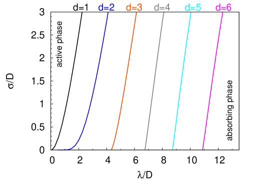
Figure 1: Phase diagram of the OBA model (1.1) ensuing from the nonperturbative renormalization group (NPRG) in dimensions $d=1,\ldots,6$, from Canet et al. [7]. For each dimension, the active phase lies on the left and the absorbing phase on the right of the transition line. For $d>2$ this line comes into the $\lambda/D$ axis at some threshold value $\lambda_{\rm c}/D$ with a finite slope $\alpha_{\rm NPRG}\approx 2.3$. The spacing between the phase transition lines for two successive dimensions is $\Delta_{\rm NPRG}\approx 2.2$.

First of all Eq. (2.19) implies the existence for large enough $\lambda$ of an absorbing region in the phase diagram, which is in full agreement with the NPRG results of Fig. 1. Furthermore, as the spatial dimension $d$ tends to infinity, so does the lattice coordination number $c$ (typically linearly with $d$), and Eq. (2.19) shows that the region of phase space to which our proof applies, recedes to infinity as $c\to\infty$. This, too, corroborates the NPRG results of Ref. [7] which indicate that an absorbing phase exists in all finite dimensions. It also matches with standard MF theory, which has effectively $d=\infty$, and no absorbing phase in this limit.

One can take a further step and analyze the shape of the phase transition line between the active and absorbing phases obtained in the SS-OBA model. As shown in the next section, it fits with the NPRG results even on a quantitative level.

2.4 Analysis of the phase diagram

In this section we analyze in greater details the location of the phase transition line in the $(\lambda/D,\sigma/D)$ plane defined by Eq. (2.19). We show that it intersects the $\lambda/D$ axis at some finite value $\lambda/D=\lambda_{\rm c}/D$, and with a positive slope. To do so we determine $\mu_{1}(\tilde{\sigma},\tilde{D})$ for arbitrary $\tilde{D}$ perturbatively in small $\tilde{\sigma}$. To linear order in $\tilde{\sigma}$, the result, derived in the Appendix, is

$$\mu_{1}(\tilde{\sigma},\tilde{D})=\tilde{D}-\frac{\tilde{D}-1}{\tilde{D}+1}\,\tilde{\sigma}\,+{\cal O}(\tilde{\sigma}^{2}).$$ (2.20)

Combining this expression with criterion (2.17) we see that for $\tilde{\sigma}\to 0$, the system will tend towards an absorbing state at the condition that

$$\tilde{D}<1\qquad\mbox{or}\qquad\lambda>\lambda_{\rm c}\,,$$ (2.21)

where

$$\lambda_{\rm c}/D=c=2d,$$ (2.22)

and in which the last equality is for the case of a hypercubic $d$-dimensional lattice.

The variation of the threshold $\lambda_{\rm c}/D$ with the dimension has also been obtained [7] within NPRG. Indeed, from Fig. 1, which is for hypercubic lattices, this variation appears to be linear, $\lambda_{\rm c}/D\simeq\Delta_{\rm NPRG}d$ with the slope equal to $\Delta_{\rm NPRG}\approx 2.2$ (as estimated in [7]). This result is in very close agreement with our Eq. (2.22), which yields $\Delta=2$ for the same slope.

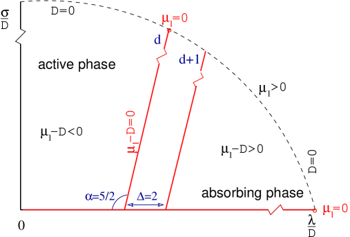
Figure 2: Phase diagram of the OBA model (1.1) according to the single-site approximation of this work, for the dimensions $d$ and $d+1$. The circle at infinity has been represented by a dashed arc. The phase transition lines come into the $\lambda/D$ axis with a slope $\alpha=\frac{5}{2}$ and for two successive dimensions have a spacing $\Delta=2$. This phase diagram is very close qualitatively and quantitatively to the one of Fig. 1.

The second order correction in $\tilde{\sigma}$ to $\mu_{1}$ can also be worked out, as shown in the Appendix, and allows for the determination of the slope of the transition line. To second order the smallest eigenvalue is given by

$$\mu_{1}(\tilde{\sigma},\tilde{D})=\tilde{D}-\frac{\tilde{D}-1}{\tilde{D}+1}\,\tilde{\sigma}\,+\frac{2(2\tilde{D}^{2}-3\tilde{D}-3)}{(2\tilde{D}+3)(\tilde{D}+1)^{3}}\tilde{\sigma}^{2}+{\cal O}(\tilde{\sigma}^{3}).$$ (2.23)

According to the criterion of Eq. (2.17) the phase transition line between the active and the absorbing phases is defined by the condition $\mu_{1}-\tilde{D}=0$. Substituting (2.23) in this condition, dividing out $\tilde{\sigma}$, writing $\tilde{\sigma}=(\sigma/D)(\tilde{D}/c)$, and using that $\tilde{\sigma}$, $\tilde{D}-1$, and $\lambda/D-c$ are of the same order we find

$$\frac{\sigma}{D} = \frac{(2\tilde{D}+3)(\tilde{D}+1)^{2}}{2\tilde{D}(2\tilde{D}^{2}-3\tilde{D}-3)}\,c(\tilde{D}-1)\,+\,{\cal O}\big{(}(\tilde{D}-1)^{2}\big{)}$$ (2.24)

$$= \frac{5}{2}\left(\frac{\lambda}{D}-c\right)\,+\,{\cal O}\left(\Big{(}\frac{\lambda}{D}-c\Big{)}^{2}\right),$$

which is the equation for the phase transition line near the threshold point $(\lambda/D,\sigma/D)=(c,0)$.

The slope $\alpha$ at the threshold appears to be $\alpha=\frac{5}{2}$, independently of $c$, i.e., of the dimension $d$. The value $\alpha=\frac{5}{2}$ compares favorably with the NPRG phase diagram of Fig. 1, where the phase transition lines appear to be merely drifting as the dimension grows, with a quasi-constant slope $\alpha_{\rm NPRG}$ numerically equal to $\alpha_{\rm NPRG}\approx 2.3$ [14].

Fig. 2 summarizes the results of this section and shows that our single-site approximation captures all the essential features of phase diagrams of the OBA model in $d>2$. It allows in particular to probe the dependence on the dimension, which is beyond the scope of standard MF approach.

3 Discussion

In addition to the discussion that has accompanied the above determination of the phase diagram, several points deserve some comments. We provide them here.

Order parameter.   Our first remark concerns the active state. According to Eq. (2.17) this state is characterized by the inequality $\mu_{1}-\tilde{D}<0$. In the region of the phase diagram where this inequality holds, Eq. (2.16) shows that the total particle number increases exponentially in time. Nevertheless, in this regime the average number of particles per occupied site, $\langle n\rangle_{\rm occ}$, is well defined in the limit $\tau\to\infty$. One may consider this quantity as the order parameter of the SS-OBA, but it should be emphasized that the usual order parameter is instead $\rho=q\langle n\rangle_{\rm occ}$ where $q$ is the fraction of occupied sites.

In the SS-OBA model each diffusion step takes the diffusing particle to an empty site. For the discussion of the phase diagram in the preceding sections there has been no need to specify whether this is a site that has perhaps previously been occupied or whether it is an entirely new site. Therefore the fraction $1-q$ of empty sites, and hence the usual order parameter $\rho$, remain undefined in the SS-OBA model.

Hence a calculation of $\rho$ within our approach would require further elaboration and/or modification of the model. A way to do this was pointed out by Dickman [15], but goes beyond our more restricted purpose of analytically studying the phase diagram.

Reformulation.   The SS-OBA model may be formulated in an equivalent way which preserves the original lattice structure. This reformulation requires that we distinguish between two notions that coincided in the definition of section (2.1), viz. between a “lattice site” in its usual sense and a “family” of particles: a family  consists of a particle having diffused to a (now not necessarily empty) lattice site, together with all the offspring it has generated on that site and which has never left it. Initially all particles on the same site are considered to constitute a family. Consequently, the particles on each site may at any time be partitioned into families. When a particle performs a diffusion step, it leaves its family and starts a family of its own on its arrival site, where other families may or may not already be present.

We may then replace rules (ii) and (iii) of section 2.1 by the following:

i (ii^′) Each particle can annihilate (at a rate $\lambda$ per pair) only with other members of its own family on that site.

(iii^′) Each particle performs diffusion steps to neighboring sites with a rate $D$ per transition; for coordination number $c$ this means that a particle will leave its site at a rate $cD$.

This reformulation of the SS-OBA does not change the mathematics and, in particular, leads to the same $\langle N(\tau)\rangle$ as found in section 2.2. It has the merit of bringing out clearly that two-particle annihilation in the SS-OBA model occurs under more restrictive conditions than in the original OBA model. This makes it tempting to believe that the average total particle number in the SS-OBA model is an upper bound to the same quantity in the OBA model. If true, our calculation would constitute an exact proof of the existence of an absorbing state in the OBA model. We have not, however, been able to prove this upper bound property and leave it as an open problem.

Below two dimensions.   Our final remark concerns what happens when the spatial dimension $d$ is equal to or less than the critical dimension $d_{c}=2$ for pure pair annihilation. For $d\leq d_{\rm c}$ the renormalisation group (both perturbative and nonperturbative) predicts that in the OBA model the threshold $\lambda_{\rm c}$ vanishes. In the SS-OBA model this would correspond for instance to ${\cal D}_{\rm c}(0)\to\infty$ in Eq. (2.19) for $d\leq 2$. We have not investigated this point further, since the behaviour of the system for small $\lambda/D$ and $\sigma/D$ corresponds to the large diffusion regime, for which we do not a priori expect the SS-OBA model to be a good description of the OBA model.

4 Conclusion

We have formulated a new approximation for reaction-diffusion problems with an absorbing-state transition. Its characteristic feature is that it forbids annihilation reactions when one or more of the participating particles have moved from the site where they were originally created. The approach then leads to what is essentially a single-site calculation, which allows the consequences to be determined analytically.

We have applied the approximation to the OBA model $A\to 2A$ and $2A\to 0$. We have shown that our theory produces qualitatively and quantitatively the main properties of its phase diagram in agreement with the predictions of nonperturbative renormalization but with far less effort.

Appendix A Appendix

We wish to calculate the smallest nonzero eigenvalue, called $-\mu_{1}(\tilde{\sigma},\tilde{D})$, of the matrix $\mathbf{M}$ defined by Eq. (2.4). We will perform this calculation for arbitrary $\tilde{D}$ and perturbatively for small $\tilde{\sigma}$. The symbol 1 will denote the identity matrix. For any matrix $\mathbf{L}$ with rows and columns labeled by $n=0,1,2,\ldots,$ we write $\mathbf{L}^{(j)}$ for the matrix obtained from it by erasing its rows and columns of indices $n=0,1,\ldots,j-1$; and we denote by $[\mathbf{L}]_{mm^{\prime}}$ the matrix obtained from it by erasing the row $m$ and column $m^{\prime}$. Hence $\mathbf{M}^{(0)}=\mathbf{M}$ and $\mathbf{M}^{(1)}=[\mathbf{M}]_{00}$.

If we modify the matrix $\mathbf{M}$ by suppressing its subdiagonal (of elements $0,\tilde{\sigma},2\tilde{\sigma},3\tilde{\sigma},\ldots$), it becomes upper triangular. This modified matrix has eigenvalues $-\nu_{k}$ given by its diagonal elements, i.e.,

$$\nu_{k}=k\tilde{D}+k\tilde{\sigma}+\tfrac{1}{2}k(k-1)\equiv\nu_{k}^{(0)}+k\tilde{\sigma},\qquad k=0,1,2,\ldots.$$ (A.1)

Hence its smallest nonzero eigenvalue is $\nu_{1}=\tilde{D}+\tilde{\sigma}$. Restoring now the subdiagonal will change the $\nu_{k}$ and we will calculate this change perturbatively to second order in $\tilde{\sigma}$. That is, we will look for a solution $\mu=\mu_{1}$ of Eq. (A.5) which has the form

$$\mu_{1}=\nu_{1}+\Delta\nu_{1}$$ (A.2)

with

$$\Delta\nu_{1}\equiv\nu_{1}^{(1)}\tilde{\sigma}+\nu_{1}^{(2)}\tilde{\sigma}^{2}+{\cal O}(\tilde{\sigma}^{3}).$$ (A.3)

The nonzero eigenvalues $\mu$ of $\mathbf{M}$ satisfy

$$\det\big{(}\mathbf{M}^{(1)}+\mu\mbox{\bf{1}}^{(1)}\big{)}=0.$$ (A.4)

A cofactor expansion of (A.4) along the column $n=0$ gives

$$-(\nu_{1}-\mu)\det\big{(}\mathbf{M}^{(2)}+\mu\mbox{\bf{1}}^{(2)}\big{)}-\tilde{\sigma}\det\big{(}[\mathbf{M}^{(1)}+\mu\mbox{\bf{1}}^{(1)}]_{10}\big{)}=0,$$ (A.5)

whence, after we substitute (A.2) in (A.5),

$$\Delta\nu_{1}=\tilde{\sigma}\,\frac{\det\big{(}[\mathbf{M}^{(1)}+\mu_{1}\mbox{\bf{1}}^{(1)}]_{10}\big{)}}{\det\big{(}\mathbf{M}^{(2)}+\mu_{1}\mbox{\bf{1}}^{(2)}\big{)}}.$$ (A.6)

The first order correction $\nu_{1}^{(1)}$ follows from linearizing Eq. (A.6) in $\tilde{\sigma}$, which amounts to setting $\mu_{1}=\nu_{1}^{(0)}=\tilde{D}$ and $\tilde{\sigma}=0$ in the two determinants of the right hand side of (A.6). Both determinants then reduce to a product of diagonal elements and identical factors cancel. Using the explicit expression of $\mathbf{M}$ together with (A.3) we then get from (A.6) the first order coefficient

$$\nu_{1}^{(1)}=-\frac{2\tilde{D}}{\tilde{D}+1},$$ (A.7)

which leads to the result shown in Eq. (2.20).

The second order in $\tilde{\sigma}$ in the expansion (A.3) determines the slope at which the phase transition line comes into the $\lambda/D$ axis in the phase diagram. This second order correction requires that one computes the determinant ratio in Eq. (A.6) to linear order in $\tilde{\sigma}$. Performing a cofactor expansion of both determinants along their column $n=0$, one gets

$$\det\big{(}[\mathbf{M}^{(1)}+\mu_{1}\mbox{\bf{1}}^{(1)}]_{10}\big{)} = 2\tilde{D}\det\big{(}\mathbf{M}^{(3)}+\mu_{1}\mbox{\bf{1}}^{(3)}\big{)}$$

$$-2\tilde{\sigma}\det\big{(}[[\mathbf{M}^{(1)}+\mu_{1}\mbox{\bf{1}}^{(1)}]_{10}]_{10}\big{)},$$

$$\det\big{(}\mathbf{M}^{(2)}+\mu_{1}\mbox{\bf{1}}^{(2)}\big{)} = -(\nu_{2}-\mu_{1})\det\big{(}\mathbf{M}^{(3)}+\mu_{1}\mbox{\bf{1}}^{(3)}\big{)}$$ (A.8)

$$-2\tilde{\sigma}\det\big{(}[\mathbf{M}^{(2)}+\mu_{1}\mbox{\bf{1}}^{(2)}]_{10}\big{)}.$$

To obtain the expansions of Eqs. (A.8) to first order in $\tilde{\sigma}$, it suffices that we evaluate the two determinantal coefficients of $\tilde{\sigma}$ in the second and fourth line above to zeroth order. Furthermore, it turns out that the first order contributions of $\det\big{(}\mathbf{M}^{(3)}+\mu_{1}\mbox{\bf{1}}^{(3)}\big{)}$ in Eqs. (A.8) cancel out in the ratio (A.6), so that only the zeroth order of this determinant is actually needed as well. The zeroth order of all the determinants is again obtained by setting $\mu_{1}=\nu_{1}^{(0)}$ and $\tilde{\sigma}=0$, upon which the matrices become upper triangular and the determinants reduce to the products of diagonal elements. Finally,

$$\nu_{1}^{(2)}=\frac{2(2\tilde{D}^{2}-3\tilde{D}-3)}{(2\tilde{D}+3)(\tilde{D}+1)^{3}}.$$ (A.9)

By combining (A.2), (A.3), (A.7), and (A.9) one obtains the second order result (2.23) exploited in the main text.

References

- [1] M. Bramson and L. Gray, Z. Wahrsch. verw. Gebiete 68, 447 (1985).
- [2] P. Grassberger, F. Krause, and T. von der Twer, J. Phys. A 17, L105 (1984).
- [3] H. Takayasu and A. Y. Tretyakov, Phys. Rev. Lett. 68, 3060 (1992).
- [4] I. Jensen, Phys. Rev. E 47, R1 (1993), I. Jensen, J. Phys. A 26, 3921 (1993).
- [5] J.L. Cardy and U.C. Täuber, Phys. Rev. Lett. 77, 4780 (1996), J.L. Cardy and U.C. Täuber, J. Stat. Phys. 90, 1 (1998).
- [6] L. Canet, B. Delamotte, O. Deloubrière, and N. Wschebor, Phys. Rev. Lett. 92, 195703 (2004).
- [7] L. Canet, H. Chaté, and B. Delamotte, Phys. Rev. Lett. 92, 255703 (2004).
- [8] H. Hinrichsen, Adv. Phys. 49, 815 (2000).
- [9] U.C. Täuber, M. Howard, and B.P. Vollmayr-Lee, J. Phys. A 38, R79 (2005).
- [10] G. Ódor, Rev. of Mod. Phys. 76, 663 (2004).
- [11] L. Peliti, J. Phys. (Paris) 46,1469 (1984), B. P. Lee, J. Phys. A 27, 2633 (1994), B. P. Lee and J. L. Cardy, J. Stat. Phys. 80, 971 (1995).
- [12] R. Dickman, Phys. Rev. A 38, 2588 (1988), D. Ben Avraham and J. K hler, Phys. Rev. A 45, 8358 (1992), J. Marro and R. Dickman, Nonequilibrium phase transitions in lattice models, Cambridge University Press (1999) Cambridge.
- [13] G. Ódor, Phys. Rev. E 70, 066122 (2004).
- [14] The reaction rates defined in Eq. (1) of [7] are such that one has the correspondence . Fig. 1 has been plotted with the definition of this work.
- [15] R. Dickman (2006), private communication.