Transitions among crystal, glass, and liquid in a binary mixture with changing particle size ratio and temperature

Abstract

Using molecular dynamics simulation we examine changeovers among crystal, glass, and liquid at high density in a two dimensional binary mixture. We change the ratio between the diameters of the two components and the temperature. The transitions from crystal to glass or liquid occur with proliferation of defects. We visualize the defects in terms of a disorder variable $D_{j}(t)$ representing a deviation from the hexagonal order for particle $j$. The defect structures are heterogeneous and are particularly extended in polycrystal states. They look similar at the crystal-glass crossover and at the melting. Taking the average of $D_{j}(t)$ over the particles, we define a disorder parameter $D(t)$, which conveniently measures the degree of overall disorder. Its relaxation after quenching becomes slow at low temperature in the presence of size dispersity. Its steady state average is small in crystal and large in glass and liquid.

I Introduction

The phase behavior of binary particle systems is much more complicated than that of one component systems, where the temperature $T$, the average number density $n=N/V$, and the composition are natural control parameters. At high densities, it is known to be profoundly influenced also by the size ratio $\sigma_{1}/\sigma_{2}$ between the diameters of the two components, $\sigma_{1}$ and $\sigma_{2}$ Dick ; Madden ; Likos ; Ito ; Stanley . If $\sigma_{1}/\sigma_{2}$ is close to unity at large $n$, the system becomes a crystal at low $T$ or a liquid at high $T$. If $\sigma_{1}/\sigma_{2}$ considerably deviates from unity, glass states are realized at large $n$ and at low $T$. In glass states, the particle motions are nearly frozen and the structural relaxation time grows, but the particle configurations are random yielding the structure factors similar to those in liquid.

Recently, the liquid-glass transition has been studied in a large number of molecular dynamics simulations on model binary mixtures both in two and three dimensions Muranaka ; Hurley ; yo ; kob ; Barrat . In these simulations, the temperature $T$ has mostly been the control parameter at fixed average density and composition. Some authors have applied a shear rate or a stress to glassy systems as a new control parameter yo ; Barrat . The size ratio $\sigma_{1}/\sigma_{2}$ has been chosen at particular values to realize fully frustrated particle configurations and to avoid crystallization and phase separation. However, for weaker size dispersity, the degree of disorder should become smaller. Polycrystals will be realized at some stage and a crystal with a small number of point defects will be reached eventually. On this crossover we are not aware of any systematic study and have no clear picture.

In this paper, we first aim to visualize the disorder brought about by the size dispersity in two dimensions (2D). To this end we will introduce a disorder variable $D_{j}(t)\geq 0$ representing a deviation of the hexagonal crystal order around each particle $j$. Snapshots of $D_{j}(t)$ realized by each simulation run will exhibit patterns indicating the nature of the defect structure. We shall observe point defects in crystal, grain boundaries in polycrystal, and amorphous disorder in glass. The average $D(t)=\sum_{j=1}^{N}D_{j}(t)/N$ over the particles is a single ”disorder parameter” characterizing the degree of overall disorder.

Halperin and Nelson NelsonTEXT found that defects play a key role in 2D melting in one component systems, predicting continuous transitions with an intermediate ”hexatic” phase between crystal and liquid. They introduced a sixfold orientation order variable, written as $\chi_{j}$ in this paper. The correlation function $g_{6}(r)$ of the thermal fluctuations of $\chi_{j}$ has been used to characterize the 2D defect-mediated melting theoretically Frenkel ; Stanley ; Ito and experimentally Rice ; Maret ; Kramer ; quinn . Our disorder variable $D_{j}(t)$ will be constructed from their $\chi_{j}$, so we will visualize the defect patterns exhibited by $D_{j}(t)$ also at the melting. The problem becomes much more complex for binary mixtures, where the crystal-liquid transition occurs with changing $T$ or $n$ at weak size dispersity Stanley ; Ito and the glass-liquid transition occurs at stronger size dispersity Muranaka ; Hurley ; yo ; kob ; Barrat . We should understand the defect structure by changing $\sigma_{1}/\sigma_{2}$ and $T$ (and/or $n$) both at the crystal-glass and crystal-liquid transitions cg .

In Sec II, we will introduce the quantities mentioned above and present our numerical results at fixed density and composition, where the defects involved in the crystal-glass and crystal-liquid transitions will be visualized. We will also calculate the overall disorder parameter $D(t)$ in transient states and in steady states as a function of $\sigma_{1}/\sigma_{2}$ and $T$. In Sec III, we will summarize our results and give some remarks.

II Numerical results

II.1 Method

We used a 2D model binary mixture interacting via a truncated Lenard-Jones (LJ) potential $v_{\alpha\beta}(r)$, where $\alpha,\beta=1,2$ represent the particle species. If the distance $r$ between two particles is larger than a cut-off $r_{\rm cut}$, we set $v_{\alpha\beta}(r)=0$. If $r<r_{\rm cut}$, it is given by the Lennard-Jones potential,

$$v_{\alpha\beta}(r)=4\epsilon\left[\left(\frac{\sigma_{\alpha\beta}}{r}\right)^{12}-\left(\frac{\sigma_{\alpha\beta}}{r}\right)^{6}\right]-C_{\alpha\beta},$$ (1)

which is characterized by the energy $\epsilon$ and the soft-core diameter $\sigma_{\alpha\beta}=(\sigma_{\alpha}+\sigma_{\beta})/2$ with $\sigma_{1}$ and $\sigma_{2}$ representing the (soft-core) diameters of the two components. The constant $C_{\alpha\beta}$ ensures $v_{\alpha\beta}(r)\rightarrow 0$ as $r\rightarrow r_{\rm cut}$, so the potential is continuous at the cut-off distance. We set $r_{\rm cut}=3.2\sigma_{1}$ for any $\alpha$ and $\beta$ note2 . The particle numbers of the two species are $N_{1}=N_{2}=500$, so $N=N_{1}+N_{2}=10^{3}$. With varying the size ratio $\sigma_{2}/\sigma_{1}$, the system volume $V$ was changed such that the volume fraction of the soft-core regions defined by

$$\phi=(N_{1}\sigma_{1}^{2}+N_{2}\sigma_{2}^{2})/V$$ (2)

was fixed at $0.9$ mostly. We set $\phi=1$ only in one case (in the lower panel of Fig.8). With the mass ratio being $m_{1}/m_{2}=(\sigma_{1}/\sigma_{2})^{2}$, we integrated the Newton equations using the leapfrog algorithm under the periodic boundary condition. The system temperature was controlled with the Nose-Hoover thermostat allen ; frenkelbook ; nose . The time step of integration was $0.002\tau$, where

$$\tau=\sigma_{1}\sqrt{m_{1}/\epsilon}.$$ (3)

Hereafter the time $t$ and the temperature $T$ will be measured in units of $\tau$ and $\epsilon/k_{B}$, respectively.

We first equilibrated the system in a liquid state at $T=2$ in a time interval of $10^{3}$ and then quenched it to a lower final temperature with further equilibration in a period of $t_{\rm eq}=1.1\times 10^{4}$ barker ; hamanaka . There was no appreciable time evolution in the pressure, the energy, etc in the time region $t\gtrsim 4\times 10^{3}$ (see Fig.8 as an example) equi . The particles were well mixed and no indication of phase separation was observed in the final time region.

In our study, the size ratio was in the range $1\leq\sigma_{1}/\sigma_{2}\leq 1.4$. We saw no tendency of phase separation. If $\sigma_{1}/\sigma_{2}$ is too large, phase separation will be detected HansenS ; Hobbie . We show typical particle configurations in Fig.1 at the final simulation time $t=1.2\times 10^{4}$ for (a) $\sigma_{2}/\sigma_{1}=1.1$, (b) $1.2$, (c) $1.225$, and (d) $1.4$ at $\phi=0.9$. The system length $V^{1/2}$ is (a) 35.03, (b) 36.81, (c) 37.27, and (d) 40.55 in units of $\sigma_{1}$. They represent (a) a crystal state with point defects, (b) and (c) polycrystal states, and (d) a glass state.

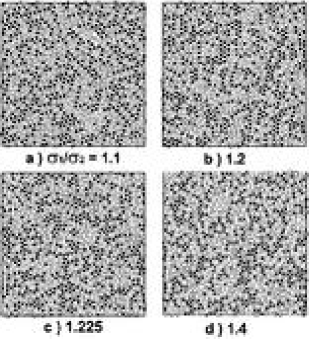
Figure 1: Particle configurations for (a) $\sigma_{1}/\sigma_{2}=1.1$, (b) 1.2, (c) 1.225, and (d) 1.4 at $\phi=0.9$ and $T=0.2$ taken at the final simulation time $t=1.2\times 10^{4}$. Smaller (larger) circles represent the smaller (larger) particles. For the visualization purpose the diameters of the circles in the snapshots are taken as $A\sigma_{1}$ and $A\sigma_{2}$ with $A<1$ for the two species.

II.2 Sixfold orientation order

In Fig.1, a large fraction of the particles are enclosed by six particles even at $\sigma_{1}/\sigma_{2}=1.4$. The particle configurations are remote from other ordered structures such as the square structure Likos . Therefore, we consider deviations from the hexagonal order. The local crystalline order is represented by a sixfold orientation order variable NelsonTEXT . For each particle $j$ we define

$$\chi_{j}=\sum_{k\in{\rm bonded}}\exp[6i\theta_{jk}],$$ (4)

where the summation is over the particles ”bonded” to the particle $j$. In our case, the two particles $j\in\alpha$ and $k\in\beta$ are bonded, if their distance $r_{jk}=|{\mbox{\boldmath$r$}}_{j}-{\mbox{\boldmath$r$}}_{k}|$ is shorter than $R_{\alpha\beta}=1.25\sigma_{\alpha\beta}$ yo . The upper cut-off $R_{\alpha\beta}$ is slightly longer than the first peak position of the pair-correlation function $g_{\alpha\beta}(r)$. The $\theta_{jk}$ is the angle of the relative vector ${\mbox{\boldmath$r$}}_{j}-{\mbox{\boldmath$r$}}_{k}$ with respect to the $x$ axis. For a perfect triangular crystal of a one component system, the complex numbers $\chi_{j}$ are all equal to $6\exp(6i\alpha)$ with $\alpha$ being the common angle of one of the crystal axes with respect to the $x$ axis. In the presence of disorder, the absolute values $|\chi_{j}|$ are significantly different from 6 for particles around defects. It is convenient to define a local crystalline angle $\alpha_{j}$ in the range $0\leq\alpha_{j}<\pi/3$ by

$$\Phi_{j}=\chi_{j}/|\chi_{j}|=e^{6i\alpha_{j}}.$$ (5)

In Fig.2, we show the snapshots of the angles $\alpha_{j}$ ($j=1,\cdots,10^{3}$) for the same particle configurations in Fig.1. The color map is illustrated in Fig.3. We can clearly see point defects, grain boundaries, and glassy particle configurations. In (b) the grain boundaries are localized, while in (c) they are percolated. Recently, using a 2D model of block copolymers, Vega et al. Vega numerically studied the grain boundary coarsening to obtain pictures of the orientation angles similar to our Fig.2, though their system corresponds to one component particle systems.

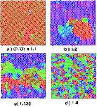
Figure 2: Snapshots of the angles $\alpha_{j}$ in Eq.(5) for (a) $\sigma_{1}/\sigma_{2}=1.1$, (b) 1.2, (c) 1.225, and (d) 1.4 with the the color map in Fig.3. The data are common to those in Fig.1. Changeover from crystal to glass occurs with polycrystal as an intermediate state.

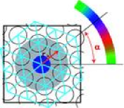
Figure 3: Color map for the angle $\alpha_{j}$ in Eq.(5) for particle $j$ at the center, around which the crystal order is perfect. The gray circle is the bonded region. The vector ${\mbox{\boldmath$r$}}_{jk}$ (red arrow) makes an angle of $\alpha_{j}=40^{\circ}$ with respect to the horizontal axis. The color of particle $j$ is then blue.

II.3 Disorder variable

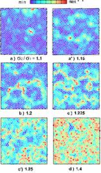
Figure 4: Disorder variable $D_{j}$ in Eq.(6) for (a) $\sigma_{2}/\sigma_{1}=1.1$, (a’) $1.15$, (b) $1.2$, (c) $1.225$, (c’) $1.25$, and (d) $1.4$ with $\phi=0.9$ and $t=1.2\times 10^{4}$. The particle configurations in (a), (b), (c), and (d) are common to those in Figs.1 and 2. Here the color changes in the order of rainbow.

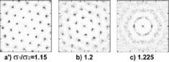
Figure 5: Structure factor for (a’) $\sigma_{2}/\sigma_{1}=1.15$, (b) $1.2$, and (b’) $1.225$ in Fig.4. Bragg peaks can be seen in (a) and (b), while it resembles to that in liquid for (c) (see (c) in Fig.7).

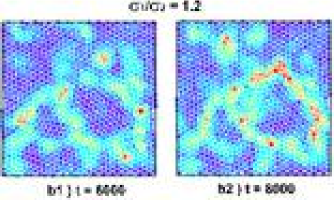
Figure 6: Disorder variable $D_{j}$ in Eq.(6) in a polycrystal state at $\sigma_{2}/\sigma_{1}=1.225$ for (b1) $t=6\times 10^{3}$ and (b2) $t=8\times 10^{3}$, in the same run giving the panel (b) in Fig.4 at $t=12\times 10^{3}$. Comparison of these three snapshots indicates very slow time evolution of the grain boundaries. See points (b1), (b2), and (b) in Fig.7 also.

We next introduce a new variable representing the degree of disorder. In terms of the difference $\Phi_{k}-\Phi_{j}$ between the bonded particle pairs, we define

$$D_{j} = {\sum_{k\in bonded}|\Phi_{j}-\Phi_{k}|^{2}}$$ (6)

$$= 2\sum_{k\in bonded}[1-\cos 6(\alpha_{j}-\alpha_{k})],$$

for each particle $j$. This quantity is called the disorder variable. If the thermal vibrations are neglected, $D_{j}$ vanishes in single-component perfect crystals and is nonvanishing around defects. It takes large values of order unity almost everywhere in highly frustrated glass states. See the comment (iv) in the last section for appropriateness of this variable in glass and liquid.

In Fig.4, snapshots of $D_{j}$ are shown for (a) $\sigma_{2}/\sigma_{1}=1.1$, (a’) $1.15$, (b) $1.2$, (c) $1.225$, (c’) $1.25$, and (d) $1.4$ at the final states of the simulation runs at $t=1.2\times 10^{4}$. Those of (a), (b), (c), and (d) are taken from the same particle configurations as in the corresponding panels of Figs.1 and 2. The color of the particles varies in the order of rainbow, being violet for $D_{j}=0$ and red for the maximum of $D_{j}$. In Fig.4, the maximum of $D_{j}$ is 1.71, 2.64, 3.59, 4.36, 4.34, and 4.58 in (a)-(d) in this order. In crystals with $\sigma_{2}/\sigma_{1}$ close to unity, a small number of defects can be detected as bright points as in (a) and (a’). In polycrystals, defects are accumulated to form grain boundaries detectable as bright closed curves enclosing small crystalline regions, as in (b) and (c). With further increasing $\sigma_{2}/\sigma_{1}$, defects are proliferated and a large fraction of the particles are depicted as bright points. In the largest size ratio in (d), most of the particles are in disordered configurations. With varying $\sigma_{2}/\sigma_{1}$, this crossover occurs in a narrow range around 1.2.

In Fig.5, the structure factor of the number density $n({\mbox{\boldmath$r$}})=n_{1}({\mbox{\boldmath$r$}})+n_{2}({\mbox{\boldmath$r$}})$ is written for (a) $\sigma_{2}/\sigma_{1}=1.15$, (b) 1.2, and (c) 1.225 to confirm the abruptness of this crystal-glass crossover. The structure factor in (a) exhibits Bragg peaks showing translational order, while that in (c) is similar to that in liquid but still retains the sixfold angular symmetry. For the intermediate case (b), the sixfold symmetry is evidently present and the translational order is being lost. (See Fig.9 below for structure factors in typical cases far from the transitions.) We note that similar structure factors were taken from a quasi 2D colloid suspension around the melting Rice .

The timescale of the particle configurations becomes exceedingly slow in glass states Muranaka ; Hurley ; yo ; kob ; Barrat . Also in polycrystal states, the motions of the grain boundaries become slow with increasing $\sigma_{2}/\sigma_{1}$, while the grain boundaries coarsen to disappear in one component systems on a rapid timescale (see the corresponding curve in Fig.7) Vega . In Fig.6, we present two additional snapshots of $D_{j}(t)$ at $\sigma_{2}/\sigma_{1}=1.225$ for $t=6\times 10^{3}$ and $t=8\times 10^{3}$, while the panel (b) in Fig.4 is the snapshot at $t=12\times 10^{3}$ in the same run. These three snapshots exhibit percolated grain boundaries with only small differences on large scales, indicating pinning of the grain boundaries. The panel (b) in Fig.2 demonstrates that the system is a polycrystal. As a result, we cannot deduce the life time of the gran boundaries from our simulation in this case.

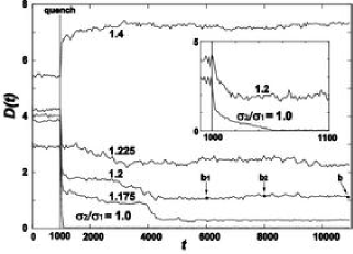
Figure 7: Relaxation of the disorder parameter $D(t)$ in Eq.(7) at $\phi=0.9$ for $\sigma_{2}/\sigma_{1}=1.0$, $1.175$, $1.2$, $1.225$, and $1.4$ from below. The temperature $T$ is lowered from 2 to 0.2 at $t=10^{3}$. For the one component case $\sigma_{2}/\sigma_{1}=1.0$, it takes place on a timescale of 50, as shown in the expanded inset. With size dispersity, $D(t)$ relaxes slowly on timescales of order $4\times 10^{3}$. Snapshots of $D_{j}(t)$ at two points (b1) and (b2) on the curve of $\sigma_{2}/\sigma_{1}=1.2$ are given in Fig.6.

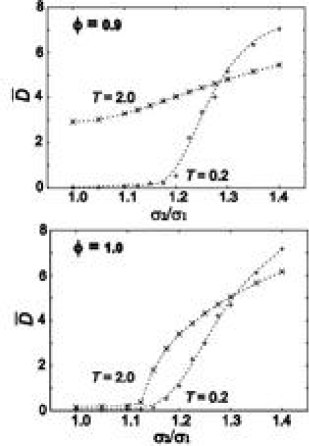
Figure 8: Disorder parameter $\bar{D}$ in Eq.(8) for $T=0.2$ and $2$, with $\phi=0.9$ in the upper panel and $1$ in the lower panel. Liquid states are realized on the curve of $T=2$ in the upper panel. The other curves show the crystal-glass crossover.

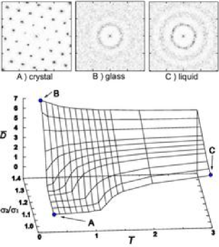
Figure 9: Disorder parameter $\bar{D}$ in Eq.(8) as a function of $\sigma_{2}/\sigma_{1}$ and $T$ for $\phi=0.9$. Typical structure factors for (A) crystal, (B) glass, and (C) liquid in the upper panel, where the corresponding points are indicated in the lower panel.

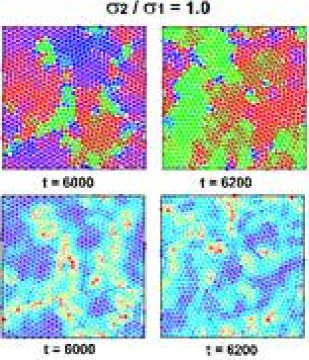
Figure 10: Polycrystal configurations of $\alpha_{j}$ in Eq.(5) (top) and $D_{j}$ in Eq.(6) (bottom) at $t=6\times 10^{3}$ (left) and $6.2\times 10^{3}$ (right) in the one component case $\sigma_{2}/\sigma_{1}=1$ at $T=1.3$ and $\phi=0.9$. The system is intermediate between crystal and liquid. The defect structure is evolving rapidly on a timescale of $50$.

II.4 Degree of overall disorder

We now introduce a single ”disorder parameter” representing the degree of overall disorder by taking the average over all the particles,

$$D(t)=\frac{1}{N}\sum_{j}D_{j}(t),$$ (7)

where the time-dependence of $D_{j}(t)$ and $D(t)$ is explicitly written. In Fig.7, we show time evolution of $D(t)$, where quenching is from liquid at $t=10^{3}$. It undergoes very slow time evolution with finite size dispersity in polycrystal and glass, in accord with Fig.6. For $\sigma_{2}/\sigma_{1}=1.4$, $D(t)$ increases upon quenching (see Fig.9 below for its reason). In the time region $t\gtrsim 4\times 10^{3}$, we can see no appreciable relaxation in these curves. For the one component case, the relaxation from liquid to crystal terminates rapidly on a timescale of 50.

However, the curves in Fig.7 with size dispersity weakly depend on time around the average even in apparent steady states. For example, $D(t)$ is 1.10 in (b1) of Fig.6, 1.17 in (b2) of Fig.6, and 1.11 in (b) of Fig.4. This temporal fluctuations should diminish for larger system size. Its deviation from the time average became largest when the grain boundaries appreciably moved in polycrystal states. For each simulation run, we defined the time average of $D(t)$ as

$${\bar{D}}=\frac{1}{t_{\rm d}}\int_{t_{\rm f}-t_{\rm d}}^{t_{\rm f}}dtD(t),$$ (8)

where $t_{\rm f}$$(=1.2\times 10^{4})$ is the terminal time of the simulation run and $t_{\rm d}(=2\times 10^{3})$ is the width of the time interval of taking data. We regard $\bar{D}$ as a steady state average though glass states may further relax on longer timescales.

In Fig.8, we plot $\bar{D}$ as a function of the size ratio. In the upper panel, where $\phi=0.9$, liquid states are realized for any $\sigma_{2}/\sigma_{1}$ at $T=2$, while the system is crystalline for $\sigma_{2}/\sigma_{1}\lesssim 1.2$ and glassy for larger $\sigma_{2}/\sigma_{1}$ at $T=0.2$. In the range $\sigma_{2}/\sigma_{1}\gtrsim 1.3$, $\bar{D}$ in the liquid state at $T=2$ becomes smaller than $\bar{D}$ in the glass state at $T=0.2$. This is because $\bar{D}$ increases weakly with increasing $\sigma_{2}/\sigma_{1}$ in liquid and increases more strongly in glass. In the lower panel, where $\phi=1$, the system crosses over from crystal to glass both for $T=0.2$ and 2, and $\bar{D}$ increases rather abruptly around $\sigma_{2}/\sigma_{1}\sim 1.2$. For $\sigma_{2}/\sigma_{1}\lesssim 1.1$, $\bar{D}$ takes a small positive number due to the thermal motions of the particles. In Fig.9, $\bar{D}$ is plotted as a function of $\sigma_{2}/\sigma_{1}$ and $T$. It shows the overall behavior of $\bar{D}$. That is, $\bar{D}$ is small in crystal and increases abruptly in glass and liquid. Interestingly, for $\sigma_{2}/\sigma_{1}>1.25$, $\bar{D}$ decreases with increasing $T$ from glass to liquid (see Fig.7). For such size ratios, highly disordered particle configurations can be pinned at low $T$ and the thermal motions at high $T$ can relax them.

II.5 Defect-mediated melting

In our simulations at fixed density, we observed defect proliferation at the melting (as well as at the crystal-glass crossover) and no coexistence of crystal and liquid regions separated by sharp interfaces. The system became highly heterogeneous (as in Fig.10 below), but no nucleation process could be detected. Figure 9 shows that $\bar{D}$ changes continuously along the $T$ axis at each $\sigma_{2}/\sigma_{1}$ including the one component limit $\sigma_{2}/\sigma_{1}=1$. Similarly, in a 2D Lenard-Jones system with $N=256$ at $\phi=0.8$, Frenkel and Mctague detected no discontinuity in the average pressure and energy Frenkel . Theoretically, the 2D melting can be either continuous or first ordrer depending the specific details of the system Saito ; Chui . It is a delicate problem to determine its precise nature in the presence of the heterogeneity developing at the transition Rice ; Maret ; Kramer ; quinn .

To visualize the physical process involved at the melting, we display snapshots of $\alpha_{j}(t)$ and $D_{j}(t)$ at $t=6000$ and 6200 in Fig.10 in the one component case at $T=1.3$, where the change of $\bar{D}$ is abrupt in Fig.9. The $D(t)$ in Eq.(7) is 1.80 at $t=6000$ and 1.60 at $t=6200$. We can see percolated grain-boundary patterns and chains of point defects. The area fraction of the crystalline regions with small $D_{j}$ continuously decreases (increases) with further raising (lowering) the temperature. We mention a simulation by McTague et al. in a one component system with soft-disk $r^{-6}$ potentials McTague , reporting the presence of both free dislocations and many grain boundaries at the melting. Some authors already pointed out relevance of grain boundaries in the 2D melting Fisher ; Chui . Using inherent-structures theory, Somer et al. Somer found percolated grain boundaries in ”inherent structures” after a hexatic-to- liquid transition. Among many experiments, grain boundaries were evidently shown in Ref.quinn .

We notice close similarity between the snapshots of the polycrystal states in Figs.6 and 10. However, very different are the timescales of the dynamics of $D_{j}(t)$ without and with size dispersity. Indeed, the patterns in Fig.10 changed appreciably on a rapid timescale of 50, while the large scale patterns in Fig.6 were nearly frozen in our simulation time.

III Summary and remarks

In summary, using MD simulation on a 2D LJ binary mixture, we have investigated the effects of the size dispersity in the range $1\leq\sigma_{1}/\sigma_{2}\leq 1.4$ and the temperature in the particle configurations at fixed average density and composition. Our main objective has been to visualize defects, so the system size ($N=10^{3}$) has been chosen to be rather small. Larger system sizes are needed to get reliable correlation functions of the density and the sixfold orientation variable.

We summarize our main results and give remarks.
(i) We have displayed the angle variable $\alpha_{j}$ defined by Eq.(5) in Fig.2 and the disorder variable $D_{j}(t)$ defined by Eq.(6) in Fig.4 at low $T=0.2$. The snapshots of these variables evidently show how the particle configurations become disordered with increasing the size ratio. Those of $D_{j}(t)$ provide the real space pictures of the defect structures on various spatial scales. We find polycrystal states with grain boundaries between crystal and glass. The motions of the grain boundaries are much slowed down with size dispersity, as in Figs.6 and 7.
(ii) The disorder parameter $D(t)$ in Eq.(7) or its time average $\bar{D}$ in Eq.(8) is a measure of overall disorder. As in Fig.7, the relaxation of $D(t)$ after quenching from a high to a low temperature occurs on a very long timescale with size dispersity, while it relaxes much faster in one component systems. The steady state average $\bar{D}$ is small in crystal and increases abruptly in glass and liquid, with increasing $\sigma_{1}/\sigma_{2}$ or $T$, as in Figs.8 and 9.
(iii) In our system, the crystal-glass and crystal-liquid crossovers proceeded with increasing the defect density without nucleation. Remarkable resemblance is noteworthy between the polycrystal patterns of $D_{j}(t)$ at the crystal-glass transition in Figs.4 and 6 and those in the one component case at the crystal-liquid transition in Fig.10. However, the timescale of the defect structure is drastically enlarged with increasing $\sigma_{1}/\sigma_{2}$. In these two transitions, the disorder parameter $\bar{D}$ increases abruptly but continuously from small (crystal) values to large (glass or liquid) values. In these cases, polycrystal states appear with large scale heterogeneities in $D_{j}(t)$, as can be seen in Figs.4, 6, and 10.
(iv) The particle configurations will increasingly deviate from the hexagonal order in the crossover from crystal to glass or liquid. They might become rather closer to other ordered structures for some fraction of the particles Ito ; Likos . In such cases, large values of $D_{j}(t)$ and $\bar{D}$ will have only qualitative meaning, since they represent deviations from the hexagonal order.
(v) We should study the pinning mechanism of grain boundaries in polycrystal in the presence of size dispersity. We should also examine the dynamical properties such as the diffusion constant, the shear viscosity, and the time-correlation functions for various degrees of disorder. They have been calculated around the liquid-glass transition Muranaka ; Hurley ; yo ; kob ; Barrat .
(vi) For the pair potentials in Eq.(1) and for our limited simulation time, we have detected no tendency of phase separation. By increasing the repulsion among the different components, we could study nucleation of crystalline domains in a glass matrix, for example.
(vii) We will report shortly on the shear flow effect at the crystal-glass and crystal-liquid transitions in 2D. It has already been studied at the liquid-glass transition yo ; Barrat . It is of interest how an applied shear affects the defect structure and induces plastic deformations OnukiPRE .

- (1) E. Dickinson and R. Parker, Chem. Phys. Lett. 79, 578 (1981).
- (2) L. Bocquet, J.P. Hansen, T. Biben, and P. Madden, J. Phys.Condensed Matter 4, 2375 (1992).
- (3) C.N. Likos and C.L. Henry, Phil. Mag. B 68, 85 (1993).
- (4) W. Vermlen and N. Ito, Phys. Rev. E 51, 4325 (1995); H. Watanabe, S. Yukawa, and N. Ito, Phys. Rev. E 71, 016702 (2005).
- (5) M. R. Sadr-Lahijany, P. Ray, and H. E. Stanley, Phys. Rev. Lett. 79, 3206 (1997).
- (6) T. Muranaka and Y. Hiwatari, Phys. Rev. E 51, R2735 (1995).
- (7) M.M. Hurley and P. Harrowell, Phys. Rev. E 52, 1694 (1995).
- (8) R. Yamamoto and A. Onuki, J. Phys. Soc. Jpn., 66 2545 (1997); Phys. Rev. E 58, 3515 (1998).
- (9) W. Kob, C. Donati, S.J. Plimton, P.H. Poole, and S.C. Glotzer, Phys. Rev. Lett. 79, 2827 (1997).
- (10) F. Varnik, L. Bocquet, and J.L. Barrat, J. Chem. Phys. 120 , 2788 (2004).
- (11) B.I. Halperin and D. R. Nelson, Phys. Rev. Lett. 41, 121 (1978); D. R. Nelson, Defects and Geometry in Condensed Matter Physics (Cambridge University Press, Cambridge, 2002), pp. 68.
- (12) D. Frenkel and J.P McTague, Phys. Rev. Lett. 42, 1632 (1979).
- (13) A.H. Marcus and S.A. Rice, Phys. Rev. E 55, 637 (1997).
- (14) K. Zahn, R. Lenke, and G. Maret, Phys. Rev. Lett. 82, 2721 (1999).
- (15) R. A. Quinn and J. Goree, Phys. Rev. E 64, 051404 (2001).
- (16) R.A. Segalman, A. Hexemer, and E.J. Kramer, Phys. Rev. Lett. 91, 196101 (2003); D. E. Angelescu, C.K. Harrison, M. L. Trawick, R. A. Register, and P. M. Chaikin, Phys. Rev. Lett. 95, 025702 (2005).
- (17) Experimentally, we need different systems to change the size ratio, so we should use ”the crystal-galss crossover” rather than ”the crystal-glass trsnsition”, to be precise.
- (18) The LJ potential among the larger particles is minimum at , which is shorter than the adopted value of even for the maximum size ratio .
- (19) M.P. Allen and D.J. Tildesley, Computer Simulation of Liquids (Clarendon Press, Oxford, 1987).
- (20) D. Frenkel and B. Smit, Understanding Molecular Simulation (Academic Press, Oxford, 1987).
- (21) S. Nóse, Molec. Phys. 52, 255 (1983).
- (22) J.A. Barker, D. Henderson, and F.F. Abraham, Physica 106A, 226 (1981).
- (23) T. Hamanaka, R. Yamamoto, and A. Onuki, Phys. Rev. E, 71, 11507 (2005).
- (24) Our simulation time becomes shorter than the structural relaxation time in glass. Furthermore, Fig.6 shows that it is shorter than the timescale of the grain boundaries at . Much longer simulation times are thus needed for more quantitative analysis of such states.
- (25) T. Biben and J. P. Hansen, Phys. Rev. Lett. 66, 2215 (1991).
- (26) E.K. Hobbie, Phys. Rev. E 55, 6281 (1997).
- (27) D. A. Vega, C.K. Harrison, D. E. Angelescu, M. L. Trawick, D. A. Huse, and P. M. Chaikin, Phys. Rev. E 71, 061803 (2005).
- (28) Y. Saito, Phys. Rev. Lett. 48, 1114 (1982).
- (29) S.T. Chui, Phys. Rev. B, 28, 178 (1983).
- (30) J.P McTague, D. Frenkel, and M.P. Allen, in Ordering in Two Dimensions, edited by S. Sinha (North-Holland, New York, 1980).
- (31) D. S. Fisher, B. I. Halperin, and R. Morf, Phys. Rev. B 20, 4692 (1979).
- (32) F.L. Sommer, Jr., G.S. Canright, T. Kaplan, K. Chen, M. Motoller, Phys. Rev. Lett. 79, 3431 (1997).
- (33) A. Onuki, Phys. Rev. E 68, 061502 (2003).