Stability of parallel/perpendicular domain boundaries in lamellar block copolymers under oscillatory shear

Synopsis

We introduce a model constitutive law for the dissipative stress tensor of lamellar phases to account for low frequency and long wavelength flows. Given the uniaxial symmetry of these phases, we argue that the stress tensor must be the same as that of a nematic but with the local order parameter being the slowly varying lamellar wavevector. This assumption leads to a dependence of the effective dynamic viscosity on orientation of the lamellar phase. We then consider a model configuration comprising a domain boundary separating laterally unbounded domains of so called parallel and perpendicularly oriented lamellae in a uniform, oscillatory, shear flow, and show that the configuration can be hydrodynamically unstable for the constitutive law chosen. It is argued that this instability and the secondary flows it creates can be used to infer a possible mechanism for orientation selection in shear experiments.

I. INTRODUCTION

Recent interest in block copolymers arises from their ability to self-assemble at the nanoscale through microphase separation and ordering, leading to mesophases with various types of symmetries, such as lamellar, cylindrical, or spherical [Fredrickson and Bates (1996); Larson (1999)]. However, when processed by thermal quench or solvent casting from an isotropic, disordered state, a macroscopic sample manifests itself as a polycrystalline configuration consisting of locally ordered but randomly oriented domains (or grains), with the presence of large amount of topological defects and unusual rheological properties. The development of the equilibrium state characterized by macroscopic orientational order, as desired in most of applications, requires unrealistically long times; hence external forces, such as steady or oscillatory shears are usually applied to accelerate domain coarsening and induce long range order. However, the mechanisms responsible for the response of the copolymer microstructure and the selection of a particular orientation over a macroscopic scale are still poorly understood. In this paper we focus on the case of imposed oscillatory shear flows on lamellar phases of block copolymers, and present an orientation selection mechanism originating from an effective viscosity contrast between lamellar phases of different orientation. Our study is based on a mesoscopic or coarse-grained description of a copolymer, but our results are expected to apply to other systems with the same symmetry as a microphase separated block copolymer.

The response of lamellar block copolymers to external shear flow can be classified according to three possible uniaxial orientations (see Fig. 1): parallel (with lamellar planes parallel to the shearing surface), perpendicular (with lamellae normal along the vorticity direction of the shear flow), and transverse (with lamellae normal directed along the shear). Solid-like or elastic response is expected for lamellar phases of transverse orientation, while fluid-like or viscous response follows for the other two, leading to different rheological properties at low shear frequencies as measured experimentally [Koppi et al. (1992); Fredrickson and Bates (1996)]. It is known that both parallel and perpendicular alignments are favored over the transverse one under shear, and either of them would be ultimately selected by shear flow, as observed in most shear aligning experiments [Larson (1999)] (although some of experimental work indicates a coexistence between parallel and transverse orientations [Pinheiro et al. (1996)], fact that might be a result of strong segregation and/or molecular entanglement). Of particular interest, and the least understood, is the selection between parallel and perpendicular orientations and the dependence on shear frequency $\omega$ and strain amplitude $\gamma$ [Koppi et al. (1992); Maring and Wiesner (1997)] as well as temperature [Koppi et al. (1992); Pinheiro and Winey (1998)]. Near the order-disorder transition temperature $T_{\rm ODT}$ and at low shear frequencies, parallel alignment has been found in poly(ethylene-propylene)-poly-(ethylethylene) (PEP-PEE) samples [Koppi et al. (1992)], while for poly(styrene)-poly-(isoprene) (PS-PI) copolymers, the observed ultimate orientation is parallel [Maring and Wiesner (1997); Leist et al. (1999)] or perpendicular [Patel et al. (1995)], depending on sample processing details such as thermal history and shear starting time [Larson (1999)]. At higher but still intermediate frequencies (where $\omega<\omega_{c}$, with $\omega_{c}$ the characteristic frequency of polymer chain relaxation dynamics), the preferred orientation is perpendicular for both PEP-PEE and PS-PI copolymers under high enough shear strain [Koppi et al. (1992); Patel et al. (1995); Maring and Wiesner (1997); Leist et al. (1999)]. At high frequencies ($\omega>\omega_{c}$) the orientation selected is different for PEP-PEE (perpendicular) than PS-PI (parallel).

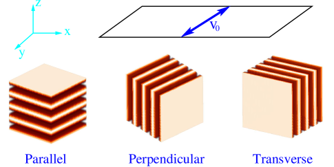
Figure 1: Three lamellar orientations (Parallel, Perpendicular, and Transverse) under shear flow.

No basic understanding exists about the mechanisms underlying the above complex phenomenology of orientation selection despite intense theoretical scrutiny in recent years. For the frequency range $\omega<\omega_{c}$ that we are interested in here, the detailed relaxation dynamics of the polymer chains within each block are not expected to be important; thus one adopts a coarse-grained, reduced description in terms of the local monomer density as the order parameter [Leibler (1980); Ohta and Kawasaki (1986); Fredrickson and Helfand (1987)]. Most of the early analyses of shear alignment of copolymers relied on thermal fluctuation effects near the transition point $T_{\rm ODT}$, and focused on the role of steady shears. A study by Cates and Milner (1989) indicates that in the vicinity of the order-disorder transition, steady shear would suppress critical fluctuations in an anisotropic manner, increase the transition temperature, and favor the perpendicular orientation. Further extension by Fredrickson (1994) by incorporating viscosity contrast between the microphases has shown that the perpendicular alignment becomes prevalent for high shear rates, while the parallel one would be favored at low shear rates.

Later consideration was given to situations that are not fluctuation dominated (such as well-aligned lamellar phases or defect structures), regarding both stability and defect dynamics. Stability differences between uniform parallel and perpendicular structures subjected to steady shears have been found [Goulian and Milner (1995)] through the consideration of anisotropic viscosities in a uniaxial fluid. Recent molecular dynamics studies as well as hydrodynamic analyses of the smectic A phase [Soddemann et al. (2004); Guo (2006)] have shown an undulation instability of parallel lamellae, as well as a transition from fully ordered parallel to perpendicular phases for large enough shear rate. Regarding the effect of oscillatory shears, an analysis of secondary instabilities [Drolet et al. (1999); Chen and Viñals (2002)] has shown that the extent of the stability region for the perpendicular orientation is always larger than that of the parallel direction, and as expected, both much larger than the transverse region. Importantly, the role of viscosity difference between the polymer blocks (as introduced by Fredrickson (1994) to address shear effects near the transition point) is found to be negligible for the stability of well-aligned lamellar structures, due to its weak coupling to long wavelength perturbations. In order to address experimental phenomena related to dynamics of structure evolution and orientation selection, more recent theoretical efforts focused on the dynamic competition between coexisting phases of different orientations. Examples include the study of a grain boundary separating parallel and transverse lamellar domains under oscillatory shears that described the dependence of the grain boundary velocity on shearing parameters such as frequency and amplitude [Huang et al. (2003); Huang and Viñals (2004)].

However, we are still far from accounting for existing experimental phenomenology on orientation selection, possibly because current approaches and models for block copolymer dynamics might not be adequate. It is important to note that block copolymer viscous response is not Newtonian even in the limit of vanishing frequency $\omega\rightarrow 0$, since Newtonian response would result in the degeneracy of parallel and perpendicular orientations, contrary to experimental findings. In the theory of Fredrickson (1994), the Newtonian assumption is used for individual microphases, with different Newtonian viscosities chosen for different monomers (blocks). We adopt here an alternative approach appropriate for flows on a scale much larger than the lamellar spacing and address the resulting deviation from Newtonian response in the low frequency limit. We introduce a constitutive law for the viscous stress tensor that explicitly incorporates the uniaxial character of lamellar phases in analogy with similar treatments of anisotropic fluids [Ericksen (1960); Leslie (1966)] and nematic liquid crystals [Forster et al. (1971); Martin et al. (1972); de Gennes and Prost (1993)]. As will be shown below, the resulting effective viscosity depends on lamellar orientation, in qualitative agreement with experiment results.

The focus of our analysis is the competition among coexisting but differently oriented lamellar domains under oscillatory shears in a polycrystalline sample. We are primarily concerned with a simplified configuration involving two regions of parallel and perpendicular orientations, and use our results to address the selection mechanism in multi domain configurations. It will be argued below that domain competition, and the orientation selection mechanism it provides, could be determined by viscosity contrast between lamellar phases due to their different orientations with respect to the imposed shear. A hydrodynamic instability is predicted at the interface separating parallel and perpendicular lamellae for certain ranges of material and shearing parameters. The resulting nonuniform secondary flows are argued to lead to the perpendicular orientation in some ranges of parameters. Comparison of our results to existing experimental findings, as well as possible examination of our predictions, are also discussed.

II. MODEL

A. Governing equations

In the range of low shear frequencies compared to the inverse of the polymer chain relaxation time, the phase behavior of a block copolymer is determined by an order parameter field $\psi$ representing the variation of local monomer density, and a velocity field ${\mathbf{v}}$. Evolution of $\psi$ is governed by a time-dependent Ginzburg-Landau equation

$$\partial\psi/\partial t+{\mathbf{v}}\cdot{\bm{\nabla}}\psi=-\Lambda\delta{\cal F}/\delta\psi,$$ (1)

with ${\cal F}$ the coarse-grained free energy given by Leibler (1980) and Ohta and Kawasaki (1986), and $\Lambda$ an Onsager kinetic coefficient. Equation (1) is coupled to the following equation governing local velocity field ${\mathbf{v}}=(v_{x},v_{y},v_{z})$ for a block copolymer system under oscillatory shear flow:

$$Re\left(\partial{\mathbf{v}}/\partial t+{\mathbf{v}}\cdot{\mathbf{\nabla}}{\mathbf{v}}\right)=-{\mathbf{\nabla}}p+{\mathbf{\nabla}}\cdot{\bm{\sigma}}^{D},$$ (2)

with the incompressibility condition ${\mathbf{\nabla}}\cdot{\mathbf{v}}=0$. Here $p$ is the pressure field, and $Re$ is the Reynolds number defined as

$$Re=\rho\omega d^{2}/\eta$$ (3)

with $\omega$ the shear frequency, $d$ the thickness of copolymer system confined between shear planes, $\rho$ the copolymer density, and $\eta$ a Newtonian viscosity. The coupling in Eqs. (1) and (2) is complex, especially when the stress tensor ${\bm{\sigma}}^{D}$ in Eq. (2) depends on the concentration field $\psi$, and when fluid inertia cannot be ignored (i.e., at nonzero Reynolds number). In order to simplify our analysis, we will assume that order parameter diffusion in Eq. (1) is negligible, so that $\psi$ is advected by the flow ${\mathbf{v}}$. At the end of the analysis, we will discuss possible implications of the flow fields obtained on order parameter diffusion as given by Eq. (1).

Equation (2) has been made dimensionless by introducing a length scale $d$, a time scale $\omega^{-1}$, and by rescaling pressure $p\rightarrow p/(\eta\omega)$. In addition to a Newtonian viscous term, Eq. (2) includes a dissipative stress tensor ${\bm{\sigma}}^{D}$ appropriate for a phase with uniaxial symmetry. We assume the constitutive equation (in dimensionless form) due to Ericksen [Ericksen (1960); Leslie (1966)] as originally derived for anisotropic fluids and later applied to a nematic liquid crystal

$$\sigma^{D}_{ij}=D_{ij}+\alpha_{1}\hat{n}_{i}\hat{n}_{j}\hat{n}_{k}\hat{n}_{l}D_{kl}+\alpha_{56}(\hat{n}_{i}\hat{n}_{k}D_{jk}+\hat{n}_{j}\hat{n}_{k}D_{ik}),$$ (4)

where $D_{ij}=\partial_{i}v_{j}+\partial_{j}v_{i}$ ($i,j=x,y,z$), but with $\hat{\mathbf{n}}=(\hat{n}_{x},\hat{n}_{y},\hat{n}_{z})$ a unit vector defining the slowly varying local normal of the lamellar phase. Eq. (4) is expected to be generic for any uniaxial phase, and thus should apply to the lamellar phases studied here by reason of symmetry. There are two independent viscosities $\alpha_{1}$ and $\alpha_{56}$ (the Leslie’s coefficients in the notation used by de Gennes and Prost (1993)), which have been rescaled as

$$\alpha_{1}\rightarrow\alpha_{1}/\eta\quad{\rm and}\quad\alpha_{56}\rightarrow\alpha_{56}/\eta.$$

They obey the relationship (due to the positivity of entropy production [Forster et al. (1971); Martin et al. (1972)])

$$\alpha_{56}\geq-1\quad{\rm and}\quad\alpha_{1}+2\alpha_{56}\geq-1.$$ (5)

For a uniform lamellar phase of parallel orientation ($\hat{\mathbf{n}}=(0,0,1)$ for the imposed shear flow along the $y$ direction considered, see Fig. 1), the Navier Stokes equation can be written explicitly as

$$Re\left(\partial_{t}v_{x}+v_{j}\partial_{j}v_{x}\right) = -\partial_{x}p+\partial_{j}^{2}v_{x}+\alpha_{56}(\partial_{z}^{2}v_{x}+\partial_{x}\partial_{z}v_{z}),$$

$$Re\left(\partial_{t}v_{y}+v_{j}\partial_{j}v_{y}\right) = -\partial_{y}p+\partial_{j}^{2}v_{y}+\alpha_{56}(\partial_{z}^{2}v_{y}+\partial_{y}\partial_{z}v_{z}),$$ (6)

$$Re\left(\partial_{t}v_{z}+v_{j}\partial_{j}v_{z}\right) = -\partial_{z}p+(1+\alpha_{56})\partial_{j}^{2}v_{z}+2(\alpha_{1}+\alpha_{56})\partial_{z}^{2}v_{z},$$

after substitution of Eq. (4) into Eq. (2). For a domain of perpendicular orientation ($\hat{\mathbf{n}}=(1,0,0)$) we have instead

$$Re\left(\partial_{t}v_{x}+v_{j}\partial_{j}v_{x}\right) = -\partial_{x}p+(1+\alpha_{56})\partial_{j}^{2}v_{x}+2(\alpha_{1}+\alpha_{56})\partial_{x}^{2}v_{x},$$

$$Re\left(\partial_{t}v_{y}+v_{j}\partial_{j}v_{y}\right) = -\partial_{y}p+\partial_{j}^{2}v_{y}+\alpha_{56}(\partial_{x}^{2}v_{y}+\partial_{x}\partial_{y}v_{x}),$$ (7)

$$Re\left(\partial_{t}v_{z}+v_{j}\partial_{j}v_{z}\right) = -\partial_{z}p+\partial_{j}^{2}v_{z}+\alpha_{56}(\partial_{x}^{2}v_{z}+\partial_{x}\partial_{z}v_{x}).$$

The Newtonian limit is recovered by setting $\alpha_{1}=\alpha_{56}=0$. Contrary to previous work on block copolymers in the creeping flow approximation [Goulian and Milner (1995); Fredrickson (1994); Chen and Viñals (2002)], we retain inertial terms in the above equations. Although small, they are significant in determining the instabilities discussed below. In the regime of small $Re$, both uniform parallel and perpendicular configurations are hydrodynamically stable as derived from Eqs. (6) and (7) with a procedure similar to that shown in Sec. III. for the grain boundary configuration.

Our assumption, Eq. (4), is consistent with experimental determinations of the loss modulus $G^{\prime\prime}$ and dynamic viscosity $\eta^{\prime}$ ($=G^{\prime\prime}/\omega$) for uniform phases of different lamellar orientations. Assuming a shear flow along $y$ (Fig. 1), we have in the creeping flow limit $Re\rightarrow 0$ (in dimensional form)

• Perpendicular ($\hat{\mathbf{n}}=(1,0,0)$): $\eta^{\prime}=\eta$;

• Parallel ($\hat{\mathbf{n}}=(0,0,1)$): $\eta^{\prime}=\eta+\alpha_{56}$;

• Transverse ($\hat{\mathbf{n}}=(0,1,0)$): $\eta^{\prime}=\eta+\alpha_{56}+\frac{2a^{2}}{(1+a^{2})^{2}}\alpha_{1}$ ($a=\gamma\sin(\omega t)$, with $\gamma$ the shear strain amplitude); when averaged over period $T$, it is $\langle\eta^{\prime}\rangle_{T}=\eta+\alpha_{56}+\frac{\gamma^{2}}{(1+\gamma^{2})^{3/2}}\alpha_{1}$.

When $\alpha_{1}>0$ and $\alpha_{56}>0$, we obtain $\eta^{\prime}_{\rm Transverse}>\eta^{\prime}_{\rm Parallel}>\eta^{\prime}_{\rm Perpendicular}$, in agreement with low $\omega$ experimental results of Koppi et al. (1992) for PEP-PEE diblock copolymers, and also with the result of molecular dynamics simulations by Guo (2006) showing smaller viscosity of perpendicular lamellae compared to that of the parallel phase. On the other hand, when $\alpha_{56}<0$, we have $\eta^{\prime}_{\rm Parallel}<\eta^{\prime}_{\rm Perpendicular}$, which is the case in PS-PI copolymers [Chen and Kornfield (1998); Gupta et al. (1995)]. The viscosity coefficients $\alpha_{1}$ and $\alpha_{56}$ could be in principle measured in block copolymers under shear flows, with experimental setups possibly similar to those used in nematic liquid crystals [see, e.g., methods reviewed by de Gennes and Prost (1993)].

B. Parallel/perpendicular configuration and viscosity contrast

We focus on coexisting lamellar domains of parallel and perpendicular orientations under oscillatory shear flows. In real samples these two types of domains may be separated by topological defects such as grain boundaries, dislocations, or disclinations. We study here the simplified configuration shown in Fig. 2, comprising two fully ordered, three-dimensional lamellar domains that are identical except for their orientation and thickness. The perpendicular domain A is of thickness $d_{A}$, and the parallel domain B of $d_{B}=1-d_{A}$ (in dimensionless form), both confined between a pair of shearing planes. The system is uniformly sheared along the $y$ direction; the velocity field ${\mathbf{v}}$ is zero on the lower boundary plane $z=0$ and equal to ${\mathbf{v}}_{0}=\gamma\cos t~{}\hat{\mathbf{y}}$ (or $\gamma\omega d\cos(\omega t)~{}\hat{\mathbf{y}}$ in dimensional form) on the upper boundary $z=1$.

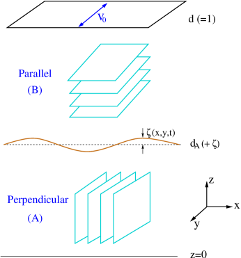
Figure 2: A parallel/perpendicular configuration subjected to oscillatory shear flow.

Under the shear considered here, bulk configurations of either orientation (parallel or perpendicular) are linearly stable. However, we will show that the configuration of Fig. 2 can become unstable. Note that the effective viscosities of the two domains are different, as discussed in Sec. A. Therefore this configuration is analogous to the case of two superposed Newtonian fluids of different viscosity, which is known to be unstable under steady (plane Couette flow [Yih (1967); Hooper (1985)]) or oscillatory [King et al. (1999)] shears. In the present case, however, the viscosity contrast follows from the orientation dependence of our constitutive law (4). This contrast between the lamellar phases can cause interface instability, but with a dependence on shearing conditions and system parameters much more complicated than that of the Newtonian limit.

III. HYDRODYNAMIC STABILITY ANALYSIS

A. Base flow

The base state for the configuration of Fig. 2 is a planar interface located at $z=d_{A}$, separating two stable perpendicular (A) and parallel (B) regions. Under uniform shear the velocity fields are along the $y$ direction: ${\mathbf{v}}_{A,B}=(0,V_{A,B},0)$. In dimensionless form, the velocities are given by

$$V_{A} = {\cal R}e\left\{\alpha_{A}\ \sinh[(1+i)\beta_{A}z]\ \gamma e^{it}\right\},$$

$$V_{B} = {\cal R}e\left\{\alpha_{A}\ \left(\sinh[(1+i)\beta_{A}d_{A}]\ \cosh[(1+i)\beta_{B}(z-d_{A})]\right.\right.$$ (8)

$$+\sqrt{m}\left.\left.\cosh[(1+i)\beta_{A}d_{A}]\ \sinh[(1+i)\beta_{B}(z-d_{A})]\ \right)\gamma e^{it}\right\},$$

with

$$\alpha_{A}^{-1}=\sinh[(1+i)\beta_{A}d_{A}]\ \cosh[(1+i)\beta_{B}d_{B}]+\sqrt{m}\cosh[(1+i)\beta_{A}d_{A}]\ \sinh[(1+i)\beta_{B}d_{B}]$$

and the viscosity ratio $m=\mu_{A}/\mu_{B}$ (with $\mu_{A}=1$ for the perpendicular region and $\mu_{B}=1+\alpha_{56}$ for a parallel domain). Here $\beta_{A}$ and $\beta_{B}$ are the inverse Stokes layer thicknesses

$$\beta_{A,B}=\left(\frac{Re}{2\mu_{A,B}}\right)^{1/2}.$$ (9)

Also for the pressure field, $p_{A}=p_{B}=p_{0}$. Note that these base state solutions are the same as those of two superposed Newtonian fluids with different viscosities $\mu_{A}$ and $\mu_{B}$ under oscillatory Couette flow [King et al. (1999)].

B. Perturbation analysis

For Newtonian fluids or in some viscoelastic models (e.g., Oldroyd-B or Maxwell fluids), the three-dimensional stability problem can be reduced to an effective two-dimensional one, with fluid stability under shear flows governed by Orr-Sommerfeld type equations for a single stream function describing two-dimensional disturbances. However, this is not the case discussed here and governed by Eqs. (2) and (4), as will be seen below.

We expand both velocity and pressure fields into the base state given above and perturbations,

$$v_{i}^{A,B}=V_{A,B}\delta_{iy}+u_{i}^{A,B}\;(i=x,y,z),\qquad p_{A,B}=p_{0}+p^{\prime}_{A,B}.$$ (10)

These flow perturbations are accompanied by an undulation of interface, denoted as $\zeta(x,y,t)$ (see Fig. 2). The boundary conditions at $z=d_{A}+\zeta(x,y,t)$ include:

Continuity of velocity

$${\mathbf{v}}^{A}={\mathbf{v}}^{B},$$ (11)

continuity of tangential stress

$$\left\{[1-(\partial_{x}\zeta)^{2}]\sigma_{xz}^{D}-\partial_{x}\zeta\ \partial_{y}\zeta\ \sigma_{yz}^{D}-\partial_{y}\zeta\ \sigma_{xy}^{D}+(\sigma_{zz}^{D}-\sigma_{xx}^{D})\partial_{x}\zeta\right\}_{A}^{B}=0,$$ (12)

$$\left\{[1-(\partial_{y}\zeta)^{2}]\sigma_{yz}^{D}-\partial_{x}\zeta\ \partial_{y}\zeta\ \sigma_{xz}^{D}-\partial_{x}\zeta\ \sigma_{xy}^{D}+(\sigma_{zz}^{D}-\sigma_{yy}^{D})\partial_{y}\zeta\right\}_{A}^{B}=0,$$ (13)

and balance of normal stress

$$\left\{-p+\sigma_{zz}^{D}-\partial_{x}\zeta\ \sigma_{xz}^{D}-\partial_{y}\zeta\ \sigma_{yz}^{D}\right\}_{A}^{B}=-\Gamma^{\prime}(\partial_{x}^{2}\zeta+\partial_{y}^{2}\zeta),$$ (14)

where $\{\}_{A}^{B}=\{\}_{B}-\{\}_{A}$, $\sigma_{ij}^{D}$ is the dissipative stress tensor, and

$$\Gamma^{\prime}=\Gamma/(\eta\omega d),$$ (15)

with $\Gamma$ the interfacial tension. Also, the kinematic condition at the interface yields

$$\left(\partial_{t}+{\mathbf{v}}^{B}\cdot{\mathbf{\nabla}}\right)\zeta=v_{z}^{B}.$$ (16)

Assume expansions of the form

$$u_{i}^{A,B}=\sum\limits_{q_{x},q_{y}}\hat{u}_{i}^{A,B}(q_{x},q_{y},z,t)\exp\left[i(q_{x}x+q_{y}y)\right],$$ (17)

where $q_{x}$ and $q_{y}$ are wave numbers in the $x$ and $y$ directions. Substituting (17) into Eqs. (6) and (7), retaining terms up to first order in the perturbation amplitudes, and eliminating the pressure, we obtain the following equations for perturbed velocity fields $\hat{u}_{z}^{A,B}$ and $\hat{u}_{x}^{A,B}$, which govern the system stability when combined with the above interfacial conditions:

For the parallel region B ($d_{A}\leq z\leq 1$),

$$Re\left[(\partial_{t}+iq_{y}V_{B})(\partial_{z}^{2}-q^{2})\hat{u}_{z}^{B}-iq_{y}(\partial_{z}^{2}V_{B})\hat{u}_{z}^{B}\right]$$

$$=(1+\alpha_{56})(\partial_{z}^{2}-q^{2})^{2}\hat{u}_{z}^{B}-2\alpha_{1}q^{2}\partial_{z}^{2}\hat{u}_{z}^{B},$$ (18)

$$Re\left[\partial_{t}(\partial_{z}^{2}-q^{2})\hat{u}_{x}^{B}+iq_{y}(\partial_{z}^{2}-q^{2})(V_{B}\hat{u}_{x}^{B})+2q_{x}q_{y}(\partial_{z}V_{B})\hat{u}_{z}^{B}\right]$$

$$=(\partial_{z}^{2}-q^{2})^{2}\hat{u}_{x}^{B}+\alpha_{56}(\partial_{z}^{2}-q^{2})\left(\partial_{z}^{2}\hat{u}_{x}^{B}-iq_{x}\partial_{z}\hat{u}_{z}^{B}\right)-2iq_{x}\alpha_{1}\partial_{z}^{3}\hat{u}_{z}^{B},$$ (19)

(here $q^{2}=q_{x}^{2}+q_{y}^{2}$), while for the perpendicular region A ($0\leq z\leq d_{A}$),

$$Re\left[(\partial_{t}+iq_{y}V_{A})(\partial_{z}^{2}-q^{2})\hat{u}_{z}^{A}-iq_{y}(\partial_{z}^{2}V_{A})\hat{u}_{z}^{A}\right]$$

$$=(\partial_{z}^{2}-q^{2})^{2}\hat{u}_{z}^{A}-\alpha_{56}q_{x}^{2}(\partial_{z}^{2}-q^{2})\hat{u}_{z}^{A}+iq_{x}[2\alpha_{1}q_{x}^{2}-\alpha_{56}(\partial_{z}^{2}-q^{2})]\partial_{z}\hat{u}_{x}^{A},$$ (20)

$$Re\left[\partial_{t}(\partial_{z}^{2}-q^{2})\hat{u}_{x}^{A}+iq_{y}(\partial_{z}^{2}-q^{2})(V_{A}\hat{u}_{x}^{A})+2q_{x}q_{y}(\partial_{z}V_{A})\hat{u}_{z}^{A}\right]$$

$$=(1+\alpha_{56})(\partial_{z}^{2}-q^{2})^{2}\hat{u}_{x}^{A}-2\alpha_{1}q_{x}^{2}(\partial_{z}^{2}-q_{y}^{2})\hat{u}_{x}^{A},$$ (21)

with rigid boundary conditions on the planes $z=0$ and $z=1$

$$\hat{u}_{x}^{A}(0)=\hat{u}_{z}^{A}(0)=\partial_{z}\hat{u}_{x}^{A}(0)=\partial_{z}\hat{u}_{z}^{A}(0)=0,$$

$$\hat{u}_{x}^{B}(1)=\hat{u}_{z}^{B}(1)=\partial_{z}\hat{u}_{x}^{B}(1)=\partial_{z}\hat{u}_{z}^{B}(1)=0.$$ (22)

The other velocity field $\hat{u}_{y}^{A,B}$ can be obtained from the incompressibility condition. Note that the form of Eqs. (18)–(21) is similar to that of the Orr-Sommerfeld equation for Newtonian fluids; however, in the above equations velocity fields are coupled (except for $q_{x}=0$), and thus the three-dimensional system here cannot be reduced to an effective two-dimensional one described by only one stream function. This irreducibility might be understood from the fact that parallel and perpendicular orientations can be distinguished only in three-dimensional space, and thus the results of the associated flows that are orientation dependent should be also three-dimensional.

The solutions to the above problem can be found by writing

$$\hat{u}_{z}^{A,B}(z,t)=e^{\sigma t}\phi_{z}^{A,B}(z,t),$$

$$\hat{u}_{x}^{A,B}(z,t)=e^{\sigma t}\phi_{x}^{A,B}(z,t),$$ (23)

$$\hat{\zeta}(t)=e^{\sigma t}h(t),$$

with interfacial perturbation $\hat{\zeta}$ defined by $\zeta(x,y,t)=\sum_{q_{x},q_{y}}\hat{\zeta}(t)\exp[i(q_{x}x+q_{y}y)]$. When $q_{y}\neq 0$, according to Floquet’s theorem $\phi_{z,x}^{A,B}$ and $h$ are periodic in time $t$ with period $T$ ($=2\pi$ here) if the eigenvalue $\sigma$ (the Floquet exponent) is simple [Yih (1968)], since coefficients in Eqs. (18)–(21) that are proportional to the base flow $V_{A,B}$ are periodic in $t$ as shown in Eq. (8). When $q_{y}=0$, $\phi_{z,x}^{A,B}$ and $h$ are time independent, and $\sigma$ represents the perturbation growth rate. In either case, the real part of $\sigma$ determines the system stability.

C. Small Reynolds number limit

The Newtonian viscosity $\eta$ is very large for block copolymers, resulting in small Reynolds numbers (Eq. (3)). For a typical block copolymer of density $\rho\sim 1$ g cm^-3 and $\eta\sim 10^{4}-10^{6}$ P, $Re/\omega\sim 10^{-4}-10^{-6}$ s for a thickness $d\sim 1$ cm. Within a reasonable range of frequencies $\omega$ of interest, we have $Re\ll 1$. The stability problem can be now solved analytically by expanding around small Reynolds number,

$$\phi_{z,x}^{A,B}(z,t)=\phi_{(z,x)0}^{A,B}(z,t)+Re\ \phi_{(z,x)1}^{A,B}(z,t)+...,$$

$$h=h_{0}(t)+Re\ h_{1}(t)+...,$$ (24)

$$\sigma=\sigma_{0}+Re\ \sigma_{1}+...,$$

with $\phi$ and $h$ functions defined in Eq. (23). Note that the order of the rescaled interfacial tension $\Gamma^{\prime}$, defined in Eq. (15) is $\omega$ dependent, and needs to be addressed separately. In the limit of $Re\rightarrow 0$ with $\Gamma^{\prime}$ finite, we set $\Gamma^{\prime}=\Gamma_{0}={\cal O}(1)$, while for small but finite values of Reynolds numbers, $\Gamma^{\prime}$ can be expressed as a power of $Re$. For a typical value of $\Gamma\sim 1$ dyne/cm (as estimated from the interfacial energy between two blocks [Helfand and Tagami (1972); Gido and Thomas (1994)]) and large $\eta$ ($\sim 10^{4}-10^{6}$ P) appropriate for block copolymers, we have $\Gamma^{\prime}\omega\sim 10^{-4}-10^{-6}$ s^-1. The intermediate range of $\omega$ (around 1 s^-1) for typical experiments leads to $\Gamma^{\prime}\equiv Re~{}\Gamma_{1}={\cal O}(Re)$, whereas for much larger frequencies $\Gamma^{\prime}/Re\ll 1$. In the following, we present the solutions of zeroth order (containing $\Gamma_{0}$) and first order (containing $\Gamma_{1}$) in $Re$, which are accurate enough to determine the stability behavior for lamellar block copolymers with typical $Re\ll 1$.

C.1 $Re\rightarrow 0$ (with $\Gamma^{\prime}=\Gamma_{0}={\cal O}(1)$)

In this parameter range, we only need the zeroth-order solution for the velocity fields, given by (for $q_{x}\neq 0$)

$$\phi_{z0}^{B} = B_{1}^{(0)}e^{b_{1}z}+B_{2}^{(0)}e^{b_{2}z}+B_{3}^{(0)}e^{b_{3}z}+B_{4}^{(0)}e^{b_{4}z},$$ (25)

$$\phi_{x0}^{B} = C_{1}^{(0)}e^{r_{1}z}+C_{2}^{(0)}e^{r_{2}z}+C_{3}^{(0)}e^{r_{3}z}+C_{4}^{(0)}e^{r_{4}z}+\frac{iq_{x}}{q^{2}}\partial_{z}\phi_{z0}^{B},$$ (26)

$$\phi_{z0}^{A} = A_{1}^{(0)}e^{a_{1}z}+A_{2}^{(0)}e^{a_{2}z}+A_{3}^{(0)}e^{a_{3}z}+A_{4}^{(0)}e^{a_{4}z}$$ (27)

$$+ D_{1}^{(0)}A_{1}^{\prime}e^{s_{1}z}+D_{2}^{(0)}A_{2}^{\prime}e^{s_{2}z}+D_{3}^{(0)}A_{3}^{\prime}e^{s_{3}z}+D_{4}^{(0)}A_{4}^{\prime}e^{s_{4}z},$$

$$\phi_{x0}^{A} = D_{1}^{(0)}e^{s_{1}z}+D_{2}^{(0)}e^{s_{2}z}+D_{3}^{(0)}e^{s_{3}z}+D_{4}^{(0)}e^{s_{4}z},$$ (28)

with

$$b_{i}^{2}=\frac{q^{2}}{\mu_{B}}\left\{\mu_{B}+\alpha_{1}\pm\left[\alpha_{1}(2\mu_{B}+\alpha_{1})\right]^{1/2}\right\},$$ (29)

$$s_{i}^{2}=\left\{\mu_{B}q^{2}+\alpha_{1}q_{x}^{2}\pm q_{x}^{2}\left[\alpha_{1}(2\mu_{B}+\alpha_{1})\right]^{1/2}\right\}/\mu_{B},$$ (30)

$$A_{i}^{\prime}=iq_{x}\left(\frac{2\alpha_{1}-\alpha_{56}^{2}}{s_{i}^{2}-q^{2}-\alpha_{56}q_{x}^{2}}-\frac{\mu_{B}}{q_{x}^{2}}\right)s_{i}$$ (31)

for $i=1,2,3,4$, and

$$r_{1}=q,\;r_{2}=-q,\;r_{3}=q/\sqrt{\mu_{B}},\;r_{4}=-q/\sqrt{\mu_{B}},$$ (32)

$$a_{1}=q,\;a_{2}=-q,\;a_{3}=\sqrt{q^{2}+\alpha_{56}q_{x}^{2}},\;a_{4}=-a_{3}.$$ (33)

For $q_{x}=0$, we have $\phi_{x0}^{A}=\phi_{x0}^{B}=0$, $\phi_{z0}^{B}$ is also given by Eq. (25), and

$$\phi_{z0}^{A}=(A_{1}^{(0)}+A_{2}^{(0)}z)e^{qz}+(-A_{1}^{(0)}+A_{3}^{(0)}z)e^{-qz}.$$ (34)

By using the boundary conditions (22), we can express the coefficients $A_{3,4}^{(0)}$, $B_{3,4}^{(0)}$, $C_{3,4}^{(0)}$, and $D_{3,4}^{(0)}$ in terms of $A_{1,2}^{(0)}$, $B_{1,2}^{(0)}$, $C_{1,2}^{(0)}$, and $D_{1,2}^{(0)}$. The remaining coefficients are obtained by solving a linear matrix equation

$${\bm{\chi}}\cdot{\bm{A}^{(0)}}={\bm{h}^{(0)}}h_{0},$$ (35)

where ${\bm{A}^{(0)}}=[A_{j}^{(0)},B_{j}^{(0)},C_{j}^{(0)},D_{j}^{(0)}]$ ($j=1,2$) for $q_{x}\neq 0$ or $[A_{j}^{(0)},B_{j}^{(0)}]$ for $q_{x}=0$, ${\bm{\chi}}$ is a $8\times 8$ or $4\times 4$ constant matrix determined by interfacial conditions (11)–(14), $h_{0}=h_{0}(t)$ denotes the $0th$-order interface perturbation, and the matrix ${\bm{h}^{(0)}}$ is a function of $\Gamma_{0}$ and $(\partial_{z}V_{B})_{0}$, with $(\partial_{z}V_{B})_{0}$ the gradient of $0th$-order base flow $V_{B}^{(0)}$:

$$V_{B}^{(0)}=[\lambda_{0}d_{A}+\delta(z-d_{A})]\gamma\cos t,\quad(\partial_{z}V_{B})_{0}=\delta\gamma\cos t,$$ (36)

with

$$\delta=m\lambda_{0},\quad\lambda_{0}=(d_{A}+md_{B})^{-1}\quad(m=\mu_{A}/\mu_{B}).$$

To lowest order, the kinematic equation (16) yields

$$\partial_{t}h_{0}=-(\sigma_{0}+iq_{y}V_{B0})h_{0}+\phi_{z0}^{B}(d_{A}),$$

where $V_{B0}=V_{B}^{(0)}(z=d_{A})=\lambda_{0}d_{A}\gamma\cos t$. From Eqs. (25) and (35), $\phi_{z0}^{B}(d_{A})$ can be expressed as

$$\phi_{z0}^{B}(d_{A})=\left[f_{z0,1}^{B}(q_{x},q_{y})\Gamma_{0}+f_{z0,2}^{B}(q_{x},q_{y})(\partial_{z}V_{B})_{0}\right]h_{0},$$ (37)

with $f_{z0,1}^{B}$ and $f_{z0,2}^{B}$ complicated but known functions of wave numbers $q_{x}$ and $q_{y}$ (and also dependent on parameters $\alpha_{1}$, $\alpha_{56}$, and $d_{A}$), and hence

$$\partial_{t}h_{0}=\left[-\sigma_{0}+f_{z0,1}^{B}(q_{x},q_{y})\Gamma_{0}\right]h_{0}+\left[-iq_{y}V_{B0}+f_{z0,2}^{B}(q_{x},q_{y})(\partial_{z}V_{B})_{0}\right]h_{0}.$$ (38)

The requirement of periodicity of $h_{0}$ with time $t$ gives the $0th$-order Floquet exponent (note that terms proportional to $V_{B0}$ and $(\partial_{z}V_{B})_{0}$ are periodic in $t$)

$$\sigma_{0}=f_{z0,1}^{B}(q_{x},q_{y})\Gamma_{0}.$$ (39)

Consequently, with initial value $h_{0}(0)$,

$$h_{0}(t) = h_{0}(0)\exp\{\int dt[-iq_{y}V_{B0}+f_{z0,2}^{B}(\partial_{z}V_{B})_{0}]\}$$ (40)

$$= h_{0}(0)\exp\left[(-iq_{y}d_{A}+mf_{z0,2}^{B})\lambda_{0}\gamma\sin t\right],$$

and the velocity fields are obtained from Eqs. (23), (25)–(28), and (35), all proportional to $h_{0}(t)$.

C.2 $Re\ll 1$, $\Gamma^{\prime}\ll 1$, such that $\Gamma^{\prime}/Re=\Gamma_{1}={\cal O}(1)$

In this case, the results of first order expansion need to be addressed. When $q_{x}\neq 0$, the solution to ${\cal O}(Re)$ yields

$$\phi_{z1}^{B} = \sum\limits_{i=1}^{4}\left[B_{i}^{(1)}e^{b_{i}z}+B^{\prime}_{i}ze^{b_{i}z}+B^{\prime}_{i+4}z^{2}e^{b_{i}z}\right],$$ (41)

$$\phi_{x1}^{B} = \sum\limits_{i=1}^{4}C_{i}^{(1)}e^{r_{i}z}+\frac{iq_{x}}{q^{2}}\partial_{z}\phi_{z1}^{B}$$ (42)

$$+ \sum\limits_{i=1}^{4}C^{\prime}_{i}ze^{r_{i}z}+\sum\limits_{i=3}^{4}C^{\prime}_{i+2}z^{2}e^{r_{i}z}+\sum\limits_{i=1}^{4}B^{\prime\prime}_{i}e^{b_{i}z},$$

$$\phi_{z1}^{A} = \sum\limits_{i=1}^{4}\left[A_{i}^{(1)}e^{a_{i}z}+D_{i}^{(1)}A^{\prime}_{i}e^{s_{i}z}+A^{\prime\prime\prime}_{i}ze^{a_{i}z}\right]+\sum\limits_{i=3}^{4}A^{\prime\prime\prime}_{i+2}z^{2}e^{a_{i}z}$$ (43)

$$+ \sum\limits_{i=1}^{4}\left[D^{\prime\prime}_{i}e^{s_{i}z}+D^{\prime\prime}_{i+4}ze^{s_{i}z}+D^{\prime\prime}_{i+8}z^{2}e^{s_{i}z}\right]$$

$$\phi_{x1}^{A} = \sum\limits_{i=1}^{4}\left[D_{i}^{(1)}e^{s_{i}z}+D^{\prime}_{i}ze^{s_{i}z}+D^{\prime}_{i+4}z^{2}e^{s_{i}z}+A^{\prime\prime}_{i}e^{a_{i}z}\right],$$ (44)

while for $q_{x}=0$, we get $\phi_{x1}^{A}=\phi_{x1}^{B}=0$, $\phi_{z1}^{B}$ given by Eq. (41), and

$$\phi_{z1}^{A} = (A_{1}^{(1)}+A_{2}^{(1)}z)e^{qz}+(-A_{1}^{(1)}+A_{3}^{(1)}z)e^{-qz}$$ (45)

$$+ (A^{\prime\prime\prime}_{1}z^{2}+A^{\prime\prime\prime}_{2}z^{3})e^{qz}+(A^{\prime\prime\prime}_{3}z^{2}+A^{\prime\prime\prime}_{4}z^{3})e^{-qz}.$$

Here exponents $b_{i}$, $r_{i}$, $a_{i}$, $s_{i}$ and coefficients $A^{\prime}_{i}$ are the same as those in Eqs. (29)–(33), and coefficients $B^{\prime}_{i}$, $B^{\prime\prime}_{i}$, $C^{\prime}_{i}$, $A^{\prime}_{i}$, $A^{\prime\prime}_{i}$, $A^{\prime\prime\prime}_{i}$, $D^{\prime}_{i}$, and $D^{\prime\prime}_{i}$ are complicated functions of $0th$ order solutions $(A^{(0)},B^{(0)},C^{(0)},D^{(0)})$. The unknown first-order coefficients $(A^{(1)},B^{(1)},C^{(1)},D^{(1)})$ can be determined by boundary conditions (22) and interfacial conditions (11)–(14), as in the above $0th$ order case. Similar to Eq. (35), the linear matrix equation governing 1st-order coefficients ${\bm{A}^{(1)}}$ ($=[A_{j}^{(1)},B_{j}^{(1)},C_{j}^{(1)},D_{j}^{(1)}]$ for $q_{x}\neq 0$, or $[A_{j}^{(1)},B_{j}^{(1)}]$ for $q_{x}=0$, with $j=1,2$) is

$${\bm{\chi}}\cdot{\bm{A}^{(1)}}={\bm{h}^{(1)}}h_{0}+{\bm{h}^{(0)}}h_{1},$$ (46)

with matrices ${\bm{\chi}}$ and ${\bm{h}^{(0)}}$ the same as those in Eq. (35), $h_{1}(t)$ the first-order interface perturbation, and the matrix ${\bm{h}^{(1)}}$ a complicated function of $\Gamma_{1}$, $(\partial_{z}V_{B})_{0}$, and $\partial_{t}(\partial_{z}V_{B})_{0}$. Thus, the solution of Eq. (46) takes the form

$${\bm{A}^{(1)}}=\left[{\bm{\chi}}^{-1}{\bm{h}^{(1)}}\right]h_{0}+\left[{\bm{A}^{(0)}}/h_{0}\right]h_{1},$$ (47)

with ${\bm{A}^{(0)}}$ given by Eq. (35), and accordingly the first-order velocity fields can be calculated with the use of Eqs. (41)-(45).

The ${\cal O}(Re)$ result of the kinematic condition (16) is given by

$$\partial_{t}h_{1}=-(\sigma_{0}+iq_{y}V_{B0})h_{1}-(\sigma_{1}+iq_{y}V_{B1})h_{0}+\phi_{z1}^{B}(d_{A}),$$ (48)

where $V_{B1}=\lambda_{2}\gamma\sin t$ is the first order base flow $V_{B}^{(1)}$ evaluated at interface $z=d_{A}$, with

$$\lambda_{2}=\frac{1}{2}(\lambda_{1}d_{A}-\lambda_{0}d_{A}^{3}/3),\quad\lambda_{1}=[(d_{A}^{3}+m^{2}d_{B}^{3})/3+md_{A}d_{B}d]\lambda_{0}^{2}.$$

The value of $\phi_{z1}^{B}(d_{A})$ is determined by solution (41), and from Eq. (47) we find

$$\phi_{z1}^{B}(d_{A})=\left[f_{z1,1}^{B}(q_{x},q_{y})\Gamma_{1}+f_{z1,2}^{B}(q_{x},q_{y})(\partial_{z}V_{B})_{0}+f_{z1,3}^{B}(q_{x},q_{y})(\partial_{z}V_{B})_{0}^{2}\right.$$

$$\left.+f_{z1,4}^{B}(q_{x},q_{y})\partial_{t}(\partial_{z}V_{B})_{0}\right]h_{0}+\left[\phi_{z0}^{B}(d_{A})/h_{0}\right]h_{1},$$ (49)

with $\phi_{z0}^{B}(d_{A})$ the $0th$-order solution as in Eq. (37), $f_{z1,1}^{B}=f_{z0,1}^{B}$, and $f_{z1,i}^{B}$ ($i=2,3,4$) obtained from first-order solution (47) and functions of $\alpha_{1}$, $\alpha_{56}$, and $d_{A}$. Substituting Eqs. (49), (36), and (39) into (48), and using the condition that $h_{1}$ is periodic in time, we obtain the first order Floquet exponent

$$\sigma_{1}=f_{z1,1}^{B}(q_{x},q_{y})\Gamma_{1}+\frac{1}{2}\delta^{2}\gamma^{2}f_{z1,3}^{B}(q_{x},q_{y}),$$ (50)

and the corresponding interface perturbation

$$h_{1}(t) = \left[h_{1}(0)/h_{0}(0)+f_{z1,2}^{B}\delta\gamma\sin t+f_{z1,3}^{B}\delta^{2}\gamma^{2}(\sin 2t)/4\right.$$ (51)

$$\left.-(iq_{y}\lambda_{2}+\delta f_{z1,4}^{B})\gamma(1-\cos t)\right]h_{0}(t),$$

with $h_{0}(t)$ given in Eq. (40). (It is convenient to choose $h_{1}(0)=0$ at time $t=0$ so that the initial condition for $h$ is $h(t=0)=h_{0}(0)$, independent of $Re$.)

Equation (50) determines stability. The first term of the r.h.s. is proportional to rescaled surface tension and is always negative, indicating the stabilizing effect of surface tension. The second term, proportional to $\gamma^{2}$, incorporates the effect of the imposed shear flow and tends to destabilize the planar boundary. Detailed results are shown in the next section.

IV. RESULTS

Given the results of the previous section, the stability of the boundary depends on the two viscosity coefficients $\alpha_{1}$ and $\alpha_{56}$, on the domain thickness $d_{A}$, the shear strain $\gamma$, as well as the Reynolds number $Re$ and the rescaled surface tension $\Gamma^{\prime}$ (both $\omega$ dependent). Here we focus on three characteristic regimes of $\Gamma^{\prime}$ (all with $Re\ll 1$ as appropriate for typical copolymers): $\Gamma^{\prime}={\cal O}(1)$, $\Gamma^{\prime}/Re={\cal O}(1)$, and $\Gamma^{\prime}/Re\ll 1$, corresponding to different ranges of shear frequencies.

A. $Re\rightarrow 0$ and $\Gamma^{\prime}={\cal O}(1)$

The first regime of interest is that of very small Reynolds number ($Re\rightarrow 0$) and finite surface tension ($\Gamma^{\prime}=\Gamma_{0}={\cal O}(1)$), which corresponds to very low frequency $\omega$ according to the analysis at the beginning of Sec. III. C. The Floquet exponent (or the perturbation growth rate) is then well approximated by zeroth-order result $\sigma_{0}$ in Eq. (39). Our calculations give $\sigma_{0}\leq 0$ (i.e., $f_{z0,1}^{B}(q_{x},q_{y})\leq 0$) for all wave numbers $q_{x}$ and $q_{y}$; thus, the system is always stable, resulting in the coexistence of parallel and perpendicular domains under shear flow. The stabilizing effect of surface tension dominates, and $\sigma_{0}\propto\Gamma_{0}$ as shown in Eq. (39).

B. $Re\ll 1$, $\Gamma^{\prime}\ll 1$, and $\Gamma^{\prime}/Re={\cal O}(1)$

In an intermediate range of $\omega$, $\Gamma^{\prime}$ is of order ${\cal O}(Re)$ as discussed in Sec. III. C. The perturbation growth rate can be written as $\sigma=Re~{}\sigma_{1}$ with the first-order exponent $\sigma_{1}$ given in Eq. (50). Note that $f_{z1,1}^{B}=f_{z0,1}^{B}\leq 0$ whereas the maximum value of $f_{z1,3}^{B}$ can be positive depending on system parameters $\alpha_{1}$, $\alpha_{56}$, and $d_{A}$, leading to a competition between the stabilizing effect of surface tension (proportional to $\Gamma_{1}=\Gamma^{\prime}/Re$) and the destabilizing influence of the imposed shear (proportional to $\gamma^{2}$). Note that $\Gamma_{1}$ can also be expressed from Eqs. (15) and (3) as

$$\Gamma_{1}=1/We=[\Gamma/(\rho d^{3})]\omega^{-2}\equiv\theta\omega^{-2},$$ (52)

with $We$ the Weber number and $\theta=\Gamma/(\rho d^{3})$. Thus, a system would be more unstable for larger shear strain $\gamma$ and frequency $\omega$.

To examine the onset of instability, we have carried out a numerical evaluation of $\sigma$ for a range of typical system parameters. For a typical copolymer system, $\rho=1$ g cm^-3, $\Gamma=1$ dyne/cm, $\eta=10^{4}$ P, and $d=1$ cm, with Reynolds number $Re=(10^{-4}{\rm s})\omega$ and rescaled surface tension $\Gamma^{\prime}=(10^{-4}{\rm s}^{-1})/\omega$. The two dimensionless viscosities are set as: $\alpha_{1}=1$, and $\alpha_{56}=-0.9$ (corresponding to an effective viscosity $\mu_{B}=1/10$ and thus a ratio $m=\mu_{A}/\mu_{B}=10$) or $\alpha_{56}=9$ (corresponding to $\mu_{B}=10$ and $m=1/10$).

Figure 3: Growth rate $\sigma/Re$ as a function of wave numbers $q_{x}$ and $q_{y}$, for $\alpha_{1}=1$, $\alpha_{56}=-0.9$, $\gamma=1$, $Re=5\times 10^{-4}$, as well as (a) $d_{A}=1/3$ (with $d_{A}/d_{B}=1/2$), with maximum growth rate $\sigma_{\rm max}=3.4\times 10^{-4}Re$ found at ${\bf q}^{\rm max}=(0,\pm 0.89)$, and (b) $d_{A}=2/3$ (with $d_{A}/d_{B}=2$), indicating that $\sigma\leq 0$ at all wavevectors.

Figure 3 shows the growth rate $\sigma_{1}=\sigma/Re$ as a function of wave numbers $(q_{x},q_{y})$, for $\alpha_{56}=-0.9$ and two different domain thicknesses $d_{A}=1/3$ (with $d_{A}/d_{B}=1/2$) and $2/3$ (with $d_{A}/d_{B}=2$). The most dangerous wave numbers are near $q_{x}=0$, as can be seen in Fig. 3a. The figure shows that the maximum growth rate ($\sigma_{\rm max}=3.4\times 10^{-4}Re$) occurs at $q_{x}^{\rm max}=0$ and $q_{y}^{\rm max}=\pm 0.89$. Results for the larger ratio $d_{A}/d_{B}=2$ are shown in Fig. 3b, indicating that the system is stable. When $\alpha_{56}=9$, we obtain opposite stability results: a small ratio $d_{A}/d_{B}=1/2$ corresponds to a stable configuration, whereas instability occurs for $d_{A}/d_{B}=2$, with $\sigma_{\rm max}$ also found at $q_{x}=0$. It is also interesting to note that at $d_{A}/d_{B}=1$, instability occurs for all values of $\alpha_{56}$ (i.e., for all effective viscosity contrast). Figure 4 shows the maximum growth rate for $\gamma=1$ and $0.5$, $\omega=5$ and $10$ (s^-1) (corresponding to $Re=5\times 10^{-4}$ and $10^{-3}$), and two different viscosities $\alpha_{56}=-0.9$ and $9$. As the shear strain amplitude $\gamma$ or frequency $\omega$ decreases, the range of unstable wavenumbers also decreases. This observation motivates the analysis of long wave solutions presented in subsection D.

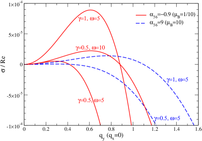
Figure 4: Growth rate $\sigma/Re$ versus $q_{y}$ at $q_{x}=0$ for $d_{A}/d_{B}=1$ and different values of $\gamma$, $\omega$, and $\alpha_{56}$.

The perturbed velocity fields are defined by Eq. (23). The velocity associated with the most unstable wavevector $(q_{x}=0,q_{y}\neq 0)$ is given by

$$\hat{u}_{x}^{\rm max}=0\quad{\rm and}\quad\hat{u}_{z}^{\rm max}=\phi_{z}\exp(\sigma_{\rm max}t),$$

with $\phi_{z}$ determined by Eqs. (25), (34), (41), and (45). Results for $\phi_{z}$ at the most unstable wavenumbers are shown in Fig. 5 (at $t=T$), and in Fig. 6 (at the interface $z=d_{A}$), for $\alpha_{1}=1$, $\gamma=1$, $Re=5\times 10^{-4}$ (with $\omega=5$ s^-1), as well as for a variety of domain thickness ratios $d_{A}/d_{B}$ and different viscosity coefficients $\alpha_{56}=-0.9$ and $9$. The corresponding interfacial perturbation $h(t)$, defined in Eq. (23), is shown in Fig. 7. Although the velocity fields near the interface are sensitive to the viscosity contrast and thickness ratios (e.g, the temporal dependence of $\phi_{z}$ for $\mu_{B}=1/10$ (with $\alpha_{56}=-0.9$) and $\mu_{B}=10$ ($\alpha_{56}=9$) is out of phase at the interface, as shown in Fig. 6), the qualitative results are the same: The instability develops around the interface, and relaxes into the perpendicular (A) and parallel (B) bulk regions. Importantly, the perturbation flow is directed along the $z$ direction (and $y$, due to the incompressibility condition), and hence it is transverse to the parallel lamellae. If the monomer density order parameter were allowed to diffuse, this secondary flow would result in the distortion of parallel lamellae, but not perpendicular.

   

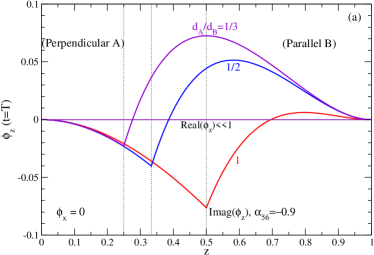
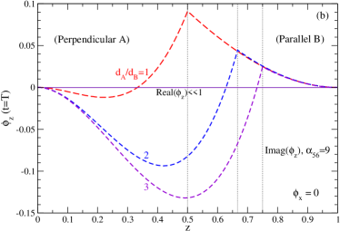
Figure 5: Spatial dependence of the velocity amplitude $\phi_{z}$ at time $t=T$ ($=2\pi$), at the most unstable wave vectors $(q_{x}^{\rm max}=0,q_{y}^{\rm max})$ given by Figs. 3 and 4. All the curves here correspond to unstable configuration with $\sigma>0$, with parameters $Re=5\times 10^{-4}$, $\alpha_{1}=1$, and $\gamma=1$. (a) $\alpha_{56}=-0.9$ ($\mu_{B}=1/10$), for $d_{A}/d_{B}=1$, $1/2$ and $1/3$; (b) $\alpha_{56}=9$ ($\mu_{B}=10$), for $d_{A}/d_{B}=1$, $2$, and $3$. The locations of domain interface are indicated by dotted lines.

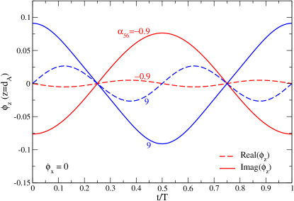
Figure 6: Temporal dependence of the velocity amplitude $\phi_{z}$ over a period $T$ at the interface $z=d_{A}$, with $d_{A}/d_{B}=1$, and other parameters the same as those of Fig. 5.

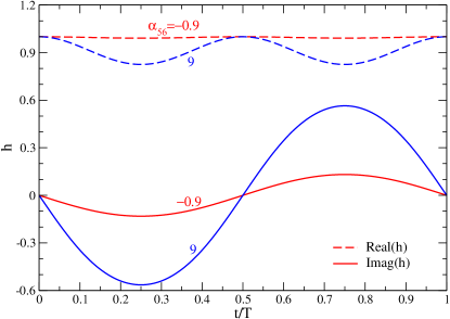
Figure 7: Temporal dependence of the interface perturbation $h$ over a period $T$, with parameters the same as those of Fig. 6.

C. $Re\ll 1$ and $\Gamma^{\prime}/Re\ll 1$

In the limit $\Gamma^{\prime}/Re\ll 1$, which corresponds to small surface tension $\Gamma$ or large enough $\omega$, the effect of the surface tension is negligible at least for solutions up to first order. This leads to $\Gamma_{0}=\Gamma_{1}=0$ in the solutions of Sec. III. Thus $\sigma_{0}=0$, and according to Eq. (50) the first order growth rate is

$$\sigma_{1}=\frac{1}{2}\delta^{2}\gamma^{2}f_{z1,3}^{B}(q_{x},q_{y}).$$ (53)

The function $f_{z1,3}^{B}(q_{x},q_{y})$ can be positive, and note that it is independent of shear parameters $\gamma$ and $\omega$. The growth rate is proportional to $\gamma^{2}$.

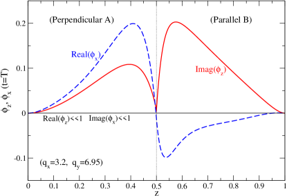
Figure 8: Velocity amplitudes $\phi_{x}$ and $\phi_{z}$ (at time $t=T$) as a function of position $z$, at the most unstable wave numbers $(q_{x}^{\rm max},q_{y}^{\rm max})=(3.2,6.95)$. The parameters are chosen as $\alpha_{56}=-0.9$, $d_{A}/d_{B}=1$, $\gamma=1$, and $Re=10^{-2}$ (corresponding to large $\omega=100$ s^-1).

A typical profile for the velocity functions $\phi_{x}$ and $\phi_{z}$ is shown in Fig. 8. In contrast with the regime discussed in subsection B ($\Gamma^{\prime}/Re=\Gamma_{1}={\cal O}(1)$), the most unstable wave numbers $q_{x}^{\rm max}$ and $q_{y}^{\rm max}$ here are both nonzero. As shown in Fig. 8 and unlike the limit discussed in subsection B, perturbed velocity fields develop along both $x$ and $z$ directions (i.e., $\phi_{x},\phi_{z}\neq 0$), leading to the distortion of both parallel and perpendicular regions. Therefore, although the parallel/perpendicular interface will move in response to the hydrodynamic instability and the resulting secondary flows, the direction of motion and hence the dominant lamellar orientation cannot be deduced from this analysis.

D. Long wave solutions

The calculations presented so far show that in the limit $Re\ll 1$, $\Gamma^{\prime}\ll 1$, with $\Gamma^{\prime}/Re={\cal O}(1)$, the wave numbers associated with instability lie at $q_{x}=0$ and small $q_{y}$, as seen in Fig. 3. Thus, we discuss next a long wave approximation to the stability analysis. We expand the solutions of Sec. III.C in powers of $q$ ($=q_{y}$ here), and find that

$$f_{z1,1}^{B}=f_{z0,1}^{B}=-f_{0}\ q^{4}+{\cal O}(q^{6}),$$ (54)

with

$$f_{0}=\frac{1}{3\Delta}d_{A}^{3}d_{B}^{3}(1+\alpha_{56}d_{A})>0,$$ (55)

and

$$f_{z1,3}^{B}=f_{1}\ q^{2}+f_{2}\ q^{4}+{\cal O}(q^{6}),$$ (56)

where

$$f_{1}=\frac{1}{60\Delta^{3}}d_{A}^{2}d_{B}^{2}\alpha_{56}f_{11}f_{12},$$ (57)

with

$$f_{11} = (1+\alpha_{56}d_{A}^{2})^{2}+4\alpha_{56}d_{A}^{2}d_{B}(1+\alpha_{56}d_{A})>0$$

$$f_{12} = (d_{A}-d_{B})(d_{A}^{2}+d_{B}^{2})+d_{A}^{8}\alpha_{56}^{4}+2d_{A}^{5}[d_{A}d_{B}^{2}+2(d_{A}-d_{B})]\alpha_{56}^{3}$$ (58)

$$+ 2d_{A}^{2}[3(d_{A}-d_{B})^{2}+(1-d_{A}^{2})^{2}-2d_{B}^{3}(1+d_{B})^{2}]\alpha_{56}^{2}$$

$$+ 2d_{A}[2(d_{A}-d_{B})^{2}+3d_{A}d_{B}^{2}-4(1+d_{A})d_{B}^{4}]\alpha_{56},$$

and $f_{2}$ a complicated but known function of $d_{A}$, $\alpha_{1}$, and $\alpha_{56}$. Here $\Delta$ is defined as

$$\Delta=(d_{B}^{2}-\mu_{B}d_{A}^{2})^{2}+4\mu_{B}d_{A}d_{B}>0.$$ (59)

Therefore, the first-order Floquet exponent (50) can be rewritten as

$$\sigma_{1} = \theta f_{z1,1}^{B}\omega^{-2}+\frac{1}{2}\delta^{2}f_{z1,3}^{B}\gamma^{2}$$ (60)

$$= \frac{1}{2}\delta^{2}f_{1}\gamma^{2}q^{2}-(\theta f_{0}\omega^{-2}-\frac{1}{2}\delta^{2}f_{2}\gamma^{2})q^{4}.$$

Thus, when $f_{1}>0$ at small $q$ we have $\sigma_{1}>0$ for all $\gamma$ and $\omega$. From the definition of $f_{1}$, we note that stability is determined by the sign of $\alpha_{56}f_{12}$ (Eqs. (57) and (58)) which is itself a function of $\alpha_{56}$ and $d_{A}$ only, and independent of shear parameters $\gamma$ and $\omega$. The calculated stability diagram of $d_{A}/d_{B}$ vs. $\mu_{B}$ ($=1+\alpha_{56}$) is shown in Fig. 9. The diagram is symmetric with respect to $d_{A}/d_{B}\rightarrow(d_{A}/d_{B})^{-1}$ and $\mu_{B}\rightarrow\mu_{B}^{-1}$. (Note that at $d_{A}/d_{B}=1$ (i.e., $d_{A}=1/2$) instability is found for all values of $\mu_{B}$, in agreement with the numerical results in subsection B.) This diagram reveals the analog of the thin layer effect in the interfacial instability caused by viscosity stratification of two superposed Newtonian fluids [Hooper (1985)]. When the thinner domain has the larger effective viscosity, instability occurs. Unlike the Newtonian case, here the effective viscosity contrast is caused by the orientation dependence of the dissipative part of the stress tensor. Note the for a polycrystalline sample, although the value of $\alpha_{56}$ ($\mu_{B}$) would be determined by the specific copolymer considered, the thickness ratio $d_{A}/d_{B}$ would vary from domain to domain. Thus, according to Fig. 9, the development of the instability would differ in different portions of a large sample.

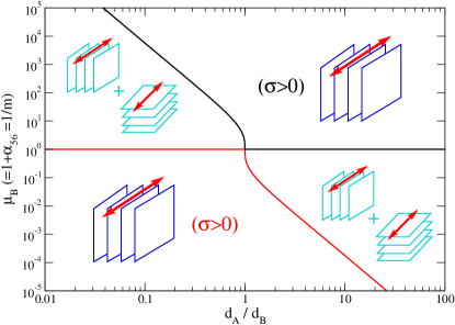
Figure 9: Stability diagram of thickness ratio $d_{A}/d_{B}$ versus viscosity contrast $\mu_{B}$ ($=m^{-1}$). For the unstable regime with $\sigma>0$, the perpendicular phase is selected over the parallel one, while the stability leads to the coexistence of parallel and perpendicular orientations.

The largest perturbation growth rate can be obtained from Eq. (60). When $\theta f_{0}\omega^{-2}-\frac{1}{2}\delta^{2}f_{2}\gamma^{2}>0$, or

$$\gamma^{2}\omega^{2}<\frac{2\theta f_{0}}{\delta^{2}f_{2}},$$ (61)

we obtain

$$\sigma_{1}^{\rm max} = \frac{\delta^{4}f_{1}^{2}}{16(\theta f_{0}-\delta^{2}f_{2}\gamma^{2}\omega^{2}/2)}\gamma^{4}\omega^{2},$$

$$q_{\rm max} = \frac{1}{2}\delta\left(\frac{f_{1}}{\theta f_{0}-\delta^{2}f_{2}\gamma^{2}\omega^{2}/2}\right)^{1/2}\gamma\omega.$$ (62)

These formulae show that both maximum growth rate and most unstable wavenumber increase with shear amplitude $\gamma$ and frequency $\omega$, in agreement with the numerical results of subsection B and Fig. 4.

V. DISCUSSION

The analysis given is purely of hydrodynamic nature and makes no reference to the response of the lamellar phases to the flows considered. The fully coupled problem is very complex, but the flow analysis conducted here can be used to argue indirectly about orientation selection. The flow perturbation ${\bf u}$ will advect the lamellae through the advection term ${\bf u}\cdot{\bm{\nabla}}\psi$ in Eq. (1), with $\psi$ the monomer concentration. Parallel lamellae are marginal to velocity fields along the $x$ and $y$ directions since these flows are parallel to the planes of constant $\psi$, but will be distorted by flows in the $z$ direction (Fig. 2). Conversely, perpendicular lamellae are unaffected by flows along either $z$ or $y$, but distorted by those along the $x$ direction. The instability mode given in Sec. IV.B for $\Gamma^{\prime}/Re={\cal O}(1)$ which might be of most experimental relevance (if we estimate the order of surface tension $\Gamma$ from the polymer-polymer interfacial energy [Helfand and Tagami (1972); Gido and Thomas (1994)], as discussed in Sec. III.C) and hence is our focus here, is associated with secondary flows with $u_{x}=0$ and $u_{z}\neq 0$; thus parallel lamellae are compressed or expanded, while the lamellar configuration in the perpendicular region remains unaffected due to the absence of modulation along its normal. Distortion of parallel lamellae would create a relative imbalance of free energy ${\cal F}$ in the two domains: ${\cal F}_{\rm Parallel}>{\cal F}_{\rm Perpendicular}$. This free energy imbalance would be relieved through the motion of the domain boundary towards the distorted parallel region. Therefore we would anticipate that a consequence of the shear flow and the resulting interfacial instabilities would be the growth of the perpendicular region at the expense of the parallel one.

Therefore, the stability diagram of Fig. 9 can be used to indirectly address orientation selection, suggesting coexistence of parallel and perpendicular domains (in the hydrodynamically stable regime) or the selection of the perpendicular orientation (in the unstable regime). It would be interesting to examine an experimental system composed of only two domains of parallel and perpendicular orientations, for verifying our predictions such as the change of instability with domain thickness ratio $d_{A}/d_{B}$ and viscosity contrast $\mu_{B}$, measuring the viscosity contrast from the location of the instability boundary, and further studying the domain evolution beyond the instability stage.

Polycrystalline samples of the type present in all shear aligning experiments involve a distribution of grain sizes and orientations. We address next how the results just obtained may provide a criterion for orientation selection under certain circumstances. Experiments [Gido et al. (1993); Qiao and Winey (2000)] reveal the presence of grain boundaries separating domains of different orientations, and we argue that the motion of these grain boundaries under the imposed shear affects the selection process. This mechanism is different than other suggestions in the literature involving grain rotation, domain instabilities, or other effects of microscopic origin that are related to block architecture (looping and bridging) [Wu et al. (2004, 2005)].

Earlier research has shown that boundaries of domains with a lamellar normal that has a component along the transverse direction will move, leading to a decrease in the size of the domain. The shear increases the free energy density of the transverse domain and originates diffusive monomer redistribution at the boundary to reduce the extent of the phase of higher free energy [Huang et al. (2003); Huang and Viñals (2004)]. Since the free energy of neither parallel nor perpendicular lamellae is affected by the shear (at least in the low frequency range of $\omega\ll\omega_{c}$ in which the Leibler [Leibler (1980)] or Ohta-Kawasaki [Ohta and Kawasaki (1986)] free energies are a good approximation), one can generally expect grain boundaries to move toward the transverse phase. Our interest in this paper is therefore in possible physical mechanisms that would account for the motion of boundaries separating domains of parallel and perpendicular orientations. According to Fig. 9, if $\alpha_{56}>0$ (as might be appropriate, for example, for PEP-PEE diblocks) an initially large perpendicular domain (A) adjacent to a smaller parallel domain (B) (so that $d_{A}/d_{B}$ is large) would grow even larger. Although our analysis does not hold beyond the linear stage of boundary deformation, it seems unlikely that any nonlinearity could saturate boundary distortion and lead to a stationary but corrugated boundary. Therefore we would predict that the perpendicular orientation will be selected for $\alpha_{56}>0$. If, on the other hand, $\alpha_{56}<0$ (as would be appropriate, for example, for PS-PI diblocks), the situation is more complicated. Instability now occurs for $d_{A}/d_{B}$ small, leading to growth of the perpendicular domain and hence to an increase of the characteristic scale $d_{A}$. To the extent that, in a sufficiently large system the boundary remains quasi-planar, the stability boundary in Fig. 9 would be reached. Once inside the stable region, any remaining curved boundaries would be expected to relax to planarity (driven by excess free energy reduction), as the planar boundary would no longer be unstable under shear. Therefore, in the case of $\alpha_{56}<0$, we would anticipate coexistence of parallel and perpendicular domains, or perhaps a dependence of the selected orientation on initial condition or sample history.

We finally examine the dependence of the largest growth rate $\sigma_{\rm max}$ on the shear amplitude $\gamma$ and angular frequency $\omega$ near the onset of instability. Note that the stability boundaries of Fig. 9 are independent of both parameters, but near onset where $\sigma\sim{\cal O}(Re)\ll 1$, experiments might detect an effective stability boundary located at the point on which $1/\sigma_{\rm max}$ is of the order of the observation time of the experiment. From Eq. (3) we have

$$\sigma_{1}^{\rm max}=\sigma_{\rm max}/Re=\sigma_{\rm max}\eta/(\rho d^{2}\omega),$$

and then given Eq. (62) we find that

$$\gamma^{2}\omega^{2}\left(\gamma^{2}\omega+\frac{8f_{2}\eta\sigma_{\rm max}}{\delta^{2}f_{1}^{2}\rho d^{2}}\right)=\frac{16\theta f_{0}\eta\sigma_{\rm max}}{\delta^{4}f_{1}^{2}\rho d^{2}},$$ (63)

with associated wavenumber

$$q_{\rm max}=\left(\frac{\eta\sigma_{\rm max}}{\theta f_{0}\rho d^{2}}\right)^{1/4}\omega^{1/4}.$$ (64)

Usually $\gamma^{2}\omega\gg 8|f_{2}|\eta\sigma_{\rm max}/(\delta^{2}f_{1}^{2}\rho d^{2})$ for very small value of $\sigma_{\rm max}$, and thus we obtain

$$\sigma_{\rm max}=\frac{\rho d^{2}\delta^{4}f_{1}^{2}}{16\theta f_{0}\eta}\gamma^{4}\omega^{3},$$ (65)

which scales as $\gamma\omega^{3/4}$ for a given block copolymer. Therefore, the line of constant $\sigma_{\rm max}$ is given by $\gamma\omega^{3/4}=const.$ This result is consistent with our numerical evaluation of solutions in Sec. III.C.2, as shown in Fig. 10 for two cases of $\alpha_{56}=-0.9$ (circles) and $9$ (diamonds). Note that the data in the log-log plot of the inset is well fitted to a straight line with slope $-3/4$. For small enough $\sigma_{\rm max}$ (e.g., $=10^{-11}$ as in Fig. 10), which is the order of the inverse experimental observation time, this line can correspond to an effective stability boundary above which the instability becomes experimentally observable.

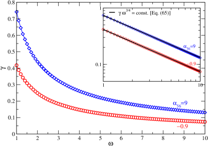
Figure 10: Lines of constant $\sigma_{\rm max}$ ($=10^{-11}$) for $d_{A}/d_{B}=1$. Symbols (circles and diamonds) are from numerical calculations, while the solid lines in the inset follow the scaling given by the long wave approximation in Eq. (65), that is, $\gamma\omega^{3/4}=const.$

To our knowledge, the only experimental determination in $\gamma$–$\omega$ space of the regions in which parallel or perpendicular lamellae are selected has been carried out for PS-PI block copolymers [Maring and Wiesner (1997); Leist et al. (1999)]. It has been found that the line separating regions of perpendicular and parallel orientations was approximately given by $\gamma\omega=const.$ No results for copolymers with $\alpha_{56}>0$ (such as PEP-PEE) are available. Given that our predictions of effective boundary only apply to this case, it would be of interest to repeat the experiments for this type of copolymers.

The above discussion corresponds to a range of shear frequency so that $\Gamma^{\prime}/Re={\cal O}(1)$. For very low frequencies so that $Re\rightarrow 0$ while $\Gamma^{\prime}={\cal O}(1)$, a parallel/perpendicular configuration is always stable due to the dominant effect of surface tension (as given in Sec. IV.A).

In combination with the stability of the lowest frequencies, our results in Fig. 10 indicate that the perpendicular orientation would be observed for large enough $\omega$ and $\gamma$. Otherwise, both parallel and perpendicular lamellae would coexist, and the selection between them would depend on experimental details such as quenched or annealed history of the sample and the starting time of the shear, as found in PS-PI copolymer samples [Patel et al. (1995); Maring and Wiesner (1997); Larson (1999)] and cannot be addressed by the stability analysis here.

VI. SUMMARY

The assumption of a dissipative part of the stress tensor $\sigma_{ij}^{D}$ which is compatible with the uniaxial symmetry of a lamellar phase leads to an effective dynamic viscosity that depends on the orientation of the lamellae relative to the shear. We expect this functional form of $\sigma_{ij}^{D}$ to capture the low frequency and long wavelength response to the lamellar phase, without making reference to the microscopic origin of the viscosity coefficients. We have explored here the consequence of this assumption on a configuration comprising parallel and perpendicular domains. Experimental evidence suggests that these two orientations are prevalent in shear aligning experiments, and we believe that the type of rheology proposed here may contribute to our understanding of the orientation selected as a function of the parameters of the block and of the shear.

In particular, we have shown that an oscillatory shear imposed on a block copolymer configuration comprising lamellar domains of parallel and perpendicular orientations can cause instability at the domain interface. The instability manifests itself by finite wavenumber undulations of the velocity field along the direction normal to parallel lamellae, which we argue would ultimately result in the growth of the perpendicular region at the expense of the parallel one. Our results indicate that the instability, and the selection of the perpendicular orientation, occur at an intermediate frequency range of small but finite value of $Re$, and depend on both viscosity contrast and domain thickness ratio. This instability is analogous to the thin layer effect in stratified fluids; that is, the system is unstable when the thinner domain is more viscous. On the other hand, at very low frequencies ($Re\rightarrow 0$), coexistence of parallel and perpendicular lamellae is found as implied by hydrodynamic stability. Also, in contrast to previous studies, the selection mechanism between parallel and perpendicular orientations introduced here is of dynamical nature, and an indirect consequence of the secondary flows generated by the hydrodynamic instability of the two-domain interface. It would be interesting to test our predictions experimentally in a test configuration of block copolymers as we have discussed here. Note that the frequency range studied here is $\omega<\omega_{c}$ in which polymer chains remain relaxed and hence the details of the individual blocks are not important. Thus our results should be independent of number and type of blocks in a copolymer.

FIGURE CAPTIONS

• Three lamellar orientations (Parallel, Perpendicular, and Transverse) under shear flow.

• A parallel/perpendicular configuration subjected to oscillatory shear flow.

• Growth rate $\sigma/Re$ as a function of wave numbers $q_{x}$ and $q_{y}$, for $\alpha_{1}=1$, $\alpha_{56}=-0.9$, $\gamma=1$, $Re=5\times 10^{-4}$, as well as (a) $d_{A}=1/3$ (with $d_{A}/d_{B}=1/2$), with maximum growth rate $\sigma_{\rm max}=3.4\times 10^{-4}Re$ found at ${\bf q}^{\rm max}=(0,\pm 0.89)$, and (b) $d_{A}=2/3$ (with $d_{A}/d_{B}=2$), indicating that $\sigma\leq 0$ at all wavevectors.

• Growth rate $\sigma/Re$ versus $q_{y}$ at $q_{x}=0$ for $d_{A}/d_{B}=1$ and different values of $\gamma$, $\omega$, and $\alpha_{56}$.

• Spatial dependence of the velocity amplitude $\phi_{z}$ at time $t=T$ ($=2\pi$), at the most unstable wave vectors $(q_{x}^{\rm max}=0,q_{y}^{\rm max})$ given by Figs. 3 and 4. All the curves here correspond to unstable configuration with $\sigma>0$, with parameters $Re=5\times 10^{-4}$, $\alpha_{1}=1$, and $\gamma=1$. (a) $\alpha_{56}=-0.9$ ($\mu_{B}=1/10$), for $d_{A}/d_{B}=1$, $1/2$ and $1/3$; (b) $\alpha_{56}=9$ ($\mu_{B}=10$), for $d_{A}/d_{B}=1$, $2$, and $3$. The locations of domain interface are indicated by dotted lines.

• Temporal dependence of the velocity amplitude $\phi_{z}$ over a period $T$ at the interface $z=d_{A}$, with $d_{A}/d_{B}=1$, and other parameters the same as those of Fig. 5.

• Temporal dependence of the interface perturbation $h$ over a period $T$, with parameters the same as those of Fig. 6.

• Velocity amplitudes $\phi_{x}$ and $\phi_{z}$ (at time $t=T$) as a function of position $z$, at the most unstable wave numbers $(q_{x}^{\rm max},q_{y}^{\rm max})=(3.2,6.95)$. The parameters are chosen as $\alpha_{56}=-0.9$, $d_{A}/d_{B}=1$, $\gamma=1$, and $Re=10^{-2}$ (corresponding to large $\omega=100$ s^-1).

• Stability diagram of thickness ratio $d_{A}/d_{B}$ versus viscosity contrast $\mu_{B}$ ($=m^{-1}$). For the unstable regime with $\sigma>0$, the perpendicular phase is selected over the parallel one, while the stability leads to the coexistence of parallel and perpendicular orientations.

• Lines of constant $\sigma_{\rm max}$ ($=10^{-11}$) for $d_{A}/d_{B}=1$. Symbols (circles and diamonds) are from numerical calculations, while the solid lines in the inset follow the scaling given by the long wave approximation in Eq. (65), that is, $\gamma\omega^{3/4}=const.$

References

- Cates and Milner (1989) Cates, M. E. and S. T. Milner, “Role of shear in the isotropic-to-lamellar transition,” Phys. Rev. Lett. 62, 1856 (1989).
- Chen and Viñals (2002) Chen, P. and J. Viñals, “Lamellar phase stability in diblock copolymers under oscillatory shear flows,” Macromolecules 35, 4183 (2002).
- Chen and Kornfield (1998) Chen, Z. R. and J. A. Kornfield, “Flow-induced alignment of lamellar block copolymer melts,” Polymer 39, 4679 (1998).
- de Gennes and Prost (1993) de Gennes, P. G. and J. Prost, The Physics of Liquid Crystals, Clarendon, Oxford (1993).
- Drolet et al. (1999) Drolet, F., P. Chen and J. Viñals, “Lamellae alignment by shear flow in a model of a diblock copolymer,” Macromolecules 32, 8603 (1999).
- Ericksen (1960) Ericksen, J. L., “Anisotropic fluids,” Arch. Ration. Mech. Anal. 4, 231 (1960).
- Forster et al. (1971) Forster, D., T. C. Lubensky, P. C. Martin, J. Swift and P. S. Pershan, “Hydrodynamics of liquid crystals,” Phys. Rev. Lett. 26, 1016 (1971).
- Fredrickson (1994) Fredrickson, G. H., “Steady shear alignment of block copolymers near the isotropic-lamellar transition,” J. Rheol. 38, 1045 (1994).
- Fredrickson and Bates (1996) Fredrickson, G. H. and F. S. Bates, “Dynamics of block copolymers,” Annu. Rev. Mater. Sci. 26, 501 (1996).
- Fredrickson and Helfand (1987) Fredrickson, G. H. and E. Helfand, “Fluctuation effects in the theory of microphase separation in block copolymers,” J. Chem. Phys. 87, 697 (1987).
- Gido et al. (1993) Gido, S. P., J. Gunther, E. L. Thomas and D. Hoffman, “Lamellar diblock copolymer grain boundary morphology. 1. Twist boundary characterization,” Macromolecules 26, 4506 (1993).
- Gido and Thomas (1994) Gido, S. P. and E. L. Thomas, “Lamellar diblock copolymer grain boundary morphology. 2. Scherk twist boundary energy calculations,” Macromolecules 27, 849 (1994).
- Goulian and Milner (1995) Goulian, M. and S. T. Milner, “Shear alignment and instability of smectic phases,” Phys. Rev. Lett. 74, 1775 (1995).
- Guo (2006) Guo, H. X., “Shear-induced parallel-to-perpendicular orientation transition in the amphiphilic lamellar phase: A nonequilibrium molecular-dynamics simulation study,” J. Chem. Phys. 124, 054902 (2006).
- Gupta et al. (1995) Gupta, V. K., R. Krishnamoorti, J. A. Kornfield and S. D. Smith, “Evolution of microstructure during shear alignment in a polystyrene-polyisoprene lamellar diblock copolymer,” Macromolecules 28, 4464 (1995).
- Helfand and Tagami (1972) Helfand, E. and Y. Tagami, “Theory of the interface between immiscible polymers. ii,” J. Chem. Phys. 56, 3592 (1972).
- Hooper (1985) Hooper, A. P., “Long-wave instability at the interface between two viscous fluids: thin layer effects,” Phys. Fluids 28, 1613 (1985).
- Huang et al. (2003) Huang, Z.-F., F. Drolet and J. Viñals, “Motion of a transverse/parallel grain boundary in a block copolymer under oscillatory shear flow,” Macromolecules 36, 9622 (2003).
- Huang and Viñals (2004) Huang, Z.-F. and J. Viñals, “Shear induced grain boundary motion for lamellar phases in the weakly nonlinear regime,” Phys. Rev. E 69, 041504 (2004).
- King et al. (1999) King, M. R., D. T. Leighton, Jr. and M. J. McCready, “Stability of oscillatory two-phase couette flow: theory and experiment,” Phys. Fluids 11, 833 (1999).
- Koppi et al. (1992) Koppi, K. A., M. Tirrell, F. S. Bates, K. Almdal and R. H. Colby, “Lamellar orientation in dynamically sheared diblock copolymer melts,” J. Phys. II (France) 2, 1941 (1992).
- Larson (1999) Larson, R. G., The Structure and Rheology of Complex Fluids, Oxford University Press, New York (1999).
- Leibler (1980) Leibler, L., “Theory of microphase separation in block copolymers,” Macromolecules 13, 1602 (1980).
- Leist et al. (1999) Leist, H., D. Maring, T. Thurn-Albrecht and U. Wiesner, “Double flip of orientation for a lamellar diblock copolymer under shear,” J. Chem. Phys. 110, 8225 (1999).
- Leslie (1966) Leslie, F. M., “Some constitutive equations for anisotropic fluids,” Quart. J. Mech. Appl. Math. 19, 357 (1966).
- Maring and Wiesner (1997) Maring, D. and U. Wiesner, “Threshold strain value for perpendicular orientation in dynamically sheared diblock copolymers,” Macromolecules 30, 660 (1997).
- Martin et al. (1972) Martin, P. C., O. Parodi and P. S. Pershan, “Unified hydrodynamic theory for crystals, liquid crystals, and normal fluids,” Phys. Rev. A 6, 2401 (1972).
- Ohta and Kawasaki (1986) Ohta, T. and K. Kawasaki, “Equilibrium morphology of block copolymer melts,” Macromolecules 19, 2621 (1986).
- Patel et al. (1995) Patel, S. S., R. G. Larson, K. I. Winey and H. Watanabe, “Shear orientation and rheology of a lamellar polystyrene-polyisoprene block copolymer,” Macromolecules 28, 4313 (1995).
- Pinheiro et al. (1996) Pinheiro, B. S., D. A. Hajduk, S. M. Gruner and K. I. Winey, “Shear-stabilized bi-axial texture and lamellar contraction in both diblock copolymer and diblock copolymer/homopolymer blends,” Macromolecules 29, 1482 (1996).
- Pinheiro and Winey (1998) Pinheiro, B. S. and K. I. Winey, “Mixed parallel-perpendicular morphologies in diblock copolymer systems correlated to the linear viscoelastic properties of the parallel and perpendicular morphologies,” Macromolecules 31, 4447 (1998).
- Qiao and Winey (2000) Qiao, L. and K. I. Winey, “Evoluton of kink bands and tilt boundaries in block copolymers at large shear strains,” Macromolecules 33, 851 (2000).
- Soddemann et al. (2004) Soddemann, T., G. K. Auernhammer, H. Guo, B. Dünweg and K. Kremer, “Shear-induced undulation of smectic-A: Molecular dynamics simulations vs. analytical theory,” Eur. Phys. J. E 13, 141 (2004).
- Wu et al. (2004) Wu, L., T. P. Lodge and F. S. Bates, “Bridge to loop transition in a shear aligned lamellae forming heptablock copolymer,” Macromolecules 37, 8184 (2004).
- Wu et al. (2005) Wu, L., T. P. Lodge and F. S. Bates, “Effect of block number on multiblock copolymer lamellae alignment under oscillatory shear,” J. Rheol. 49, 1231 (2005).
- Yih (1967) Yih, C. S., “Instability due to viscosity stratification,” J. Fluid Mech. 27, 337 (1967).
- Yih (1968) Yih, C. S., “Instability of unsteady flows or configurations: Part 1. Instability of a horizontal liquid layer on an oscillating plane,” J. Fluid Mech. 31, 737 (1968).