Effects of elasticity on the shape of measured shear signal in two-dimensional assembly of disks

Abstract

A Molecular Dynamics approach has been used to compute the shear force resulting from the shearing of disks. Two-dimensional monodisperse disks have been put in an horizontal and rectangular shearing cell with periodic boundary conditions on right and left hand sides. The shear is applied by pulling the cover of the cell either at a constant rate or by pulling a spring, linked to the cover, with a constant force. Depending on the rate of shearing and on the elasticity of the whole set up, we showed that the measured shear force signal is either irregular in time, regular in time but not in shape, or regular in shape.

I Introduction

When a macroscopically flat solid is pulled horizontally over an also macroscopically flat substrate, for given rates of pulling and of normal loads, the solid undergoes an intermittent behavior made of periods where it sticks to the substrate followed by periods where it slips over the same substrate. Several models have been written to explain this phenomenon. The first model explained this stick slip behavior by parameters of the system: the static friction and the dynamic friction coefficients and the normal load coulomb . In the years 1950, Bowden and Tabor made the theory that the friction coefficient depends on the strength of the material bowden . Moreover, Dieterich dieterich1 ; dieterich2 and Heslot et al. heslot demonstrated that the friction coefficients where not constant during one experiment, they showed that there was an aging process in the material. Finally, Baumberger baumberger showed that the transition from a continuous sliding to a stick slip behavior was dependent on the elasticity of the measuring set up. A model was introduced by Dieterich, Rice and Ruina dieterich ; ruina to give a mathematical basis to the stick slip phenomenon.

By the same way, if a granular medium is sheared by pulling an horizontal cover on the top of it, the granular system undergoes alternatively sticks (i.e. the whole system is stopped) and slips. This stick slip behavior depends on the rate at which the granular medium is pulled and on the normal load which is applied on it. Several experiments have been made on granular matter under shear as well for dry grains nasuno ; nasuno2 ; lubert ; deryck ; coste ; albert ; geng as for cohesive grains oliver .Numerical simulations have been performed on this topic by Thompson and Grest thompson .

But the question of the elasticity of all the elements setting up the shear experiment has almost not been studied. Baumberger baumberger has shown that the existence of a stick slip behavior when dragging a solid inside a granular medium, depends on the elasticity of the elastic component of the pulling set up. However, it is very difficult to estimate the elasticity of the shearing apparatus, and therefore of the grains and in case of cohesive grains, the elasticity of the interactions between neighbouring grains. A previous study olivi has shown that in the case of a numerical model of the shearing, at a constant shearing rate, of two-dimensional disks , it is possible to replace the action of the grains by one single spring. But what happens if all the components of the experimental or numerical set up have their own elasticity? In order to answer this question, we computed by a numerical model the shearing of disks in a shearing cell with non infinite and infinite elasticity, and with cohesion or without cohesion between neighbouring grains.

II Numerical Model

Molecular Dynamics is a powerful numerical method to study the dynamics of granular materials truc . The model we used here is a version of Molecular Dynamics for granular flow with cohesion in a two-dimensional shearing cell olivi ; truc ; truc2 ; olivi1 ; olivi2 . Particles are modeled as N disks that have equal density $\rho=2.2g.cm^{-2}$ and diameters $d=200\mu m$. The only external force acting on the system results from gravity, $g=981cm.s^{-2}$. The particle-particle and particle-wall contacts are described in the normal direction (i.e. in the particles’ center-center direction) by a Hooke-like force law. The normal force is written:

$${\bf f}_{n}(i,j)=(-Yr_{eff}[\frac{1}{2}(d_{i}+d_{j})-|{\bf r}_{i,j}|]+$$

$$\gamma\frac{m_{eff}({\bf v}_{i,j}.{\bf r}_{i,j})}{r_{eff}|{\bf r}_{i,j}|})\frac{{\bf r}_{i,j}}{|{\bf r}_{i,j}|}$$ (1)

where $Y$ is the Young modulus of the solid, $r_{eff}$ ($m_{eff}$) stands for the effective radius (mass) of the particles $i$ and $j$, ${\bf v_{ij}}={\bf v_{i}}-{\bf v_{j}}$ is the relative velocity of particle $j$ towards particle $i$. The effective radius is defined here as the radius of the disk which effectively enters in the interaction with another disk, it can be smaller than the real disk radius in the case where the disks overlap or larger in the case of capillary interaction (see below). The effective radius is proportional to the distance between the centers of the disks if these two are in interaction:

$$r_{eff}=\frac{(|({\bf r_{i}}-{\bf r_{j}})|)^{2}}{(d_{i}+d_{j})/4}$$ (2)

assuming that the disks never overlap more than $d_{i}/4$ and therefore adapting the time step.

The effective mass is defined here as the mass which contributes to the shearing, in our case all disks have their effective mass equal to their real mass except the disks which build the bottom of the shearing cell. $d_{i}$ (resp. $d_{j}$) is the diameter of particle $i$ (resp. $j$) and ${\bf r_{ij}}$ points from particle $i$ to particle $j$. $\gamma$ is a phenomenological dissipation coefficient.

We model the friction force between particles by putting a virtual spring at the point of first contact. Its elongation is integrated over the entire collision time and set to zero when the contact is lost. The maximum possible value of the restoring force in the shear direction (i.e. in the plane perpendicular to the normal direction), according to Coulomb’s criterion, is proportional to the normal force multiplied by the friction coefficient $\mu$. It gives a friction force ${\bf f_{s}}(i,j)$ which is written:

$${\bf f}_{s}(i,j)=-sign(f_{f}(i,j))min(f_{f}(i,j),\mu|f_{n}(i,j)|){\bf s}$$ (3)

$${\bf f}_{f}(i,j):=-\int(\dot{r}_{i}-\dot{r}_{j}){\bf s}dt$$ (4)

where $s$ stands for the unit vector in the shear direction. When a particle collides with the cylinder wall, the same forces (1) and (2) act with infinite mass and radius for particle $j$. The disks are allowed to rotate. The rotational force is given by:

$${\bf f}_{rot}=r_{eff}{\bf f}_{s}$$ (5)

Cohesive forces were modelled by adding a spring force to the normal force when particles are in contact:

$$f_{cap}=Kr_{eff}\frac{1}{2}(d_{i}+d_{j})$$ (6)

where $K$ is the corresponding elastic constant (with a dimension of a Young modulus). When the distance (proportional to the effective radius) between the surface of the particles is lower than 10 % of the diameter of the smallest particle, the value of the spring constant is multiplied by the distance between the particles. This additive force is set to zero when the elongation of the virtual spring reaches a maximum length of 10% of the smallest particle diameter.

This cohesive force is a good model for capillary forces between beads with nanoasperities.

The disks are put in an horizontal and rectangular shearing cell with or without blades, one can see an example of this shearing cell in ref.olivi . Periodic boundary conditions are imposed on the left and right hand side of the cell. Shear is applied on the disks in the shearing cell by translating the upper cover on which are linked blades to drag the disks or without any blades. The shear cell is made of disks in order to simplify the interactions of the bulk disks and the shear cell: the upper cover is made of disks of non zero effective mass (allowing the vertical move of the cover) and the bottom of the cell is made of disks with zero effective mass (allowing a stable position of the shear cell with respect to gravity). Shear is applied on the disks by translating the upper cover either at constant velocity, whatever the resistance to translation of the granular medium, or with a spring linked to the cover. In this last case, the acceleration ${\bf a_{c}}$ and force ${\bf f_{c}}$ acted by the cover on the disks assembly is given by:

$${\bf a_{c}}(t+dt)=({\bf f_{c}}(t)+K_{c}{\bf x}(t))/p_{w}$$ (7)

$${\bf x}(t+dt)={\bf x}(t)+K_{c}{\bf x}(t)$$ (8)

where $K_{c}$ is the elasticity constant of the spring pulling the cover and $p_{w}$ is the weight of the cover.

The upper cover of the cell is allowed to undergo a vertical shift, the magnitude of this shift depending on the weight of this upper cover ( and therefore on the effective mass of the upper cover disks), on the velocity of the upper cover and on the disks assembly dilation. We added no vertical elasticity to the cover as it would be more difficult to analyze the results with one more elastic component.

III Results and Discussion

The parameters of our computations were the followings: the weight of the cover was equal to $=0.552g$, the mass of one disk being equal to $2.76.10^{-3}g$. The length of the cell was $L=8mm$ and the height of the blades was $h=1mm$. We used $N=720$ disks. The dissipation coefficient was equal to $0.7m.s^{-1}$, the Young modulus was $Y=14640g.cm^{-1}.s^{-2}$ and the spring constant was $K=300g.cm^{-1}.s^{-2}$ for the case of cohesive disks. We computed the total force acted on the upper cover by the disk assembly as a resistance to shear. For this, we added only the horizontal coordinates of the forces acting on the cover. This total force is similar to a stress. The height of the cover increased after the beginning of the simulation for all cases of shear rates and elastic constants.

Results are given in figures 1, 2 , 3 and 4. These figures represent different responses of the numerical set up as a function of the cover elasticity (vertical coordinates) and shearing rates (horizontal coordinates). Each symbol corresponds to one value of the cover elasticity and one value of the shearing rate, each of them given by its coordinates. For the sake of simplicity, we gave an elasticity of 100$g.s^{-2}$ to covers with infinite elasticity as our plots are in log-log. Five regions have been identified in these plots:

• I: regular in time (with a characteristic frequency) but irregular in shape (noisy)

• II: irregular in time and irregular in shape

• III: curved slip signal and irregular in time

• IV: regular in shape and irregular in time

• V: regular in shape and in time

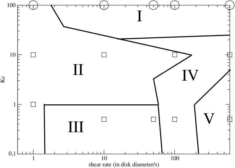
Figure 3: Diagram of the computed shear signal for a shear cell with blades and for non cohesive disks as a function of the elastic constant $K_{c}$ (in $g.s^{-2}$) of the cover and of the shear rate (in disk diameter per $s^{-1}$)

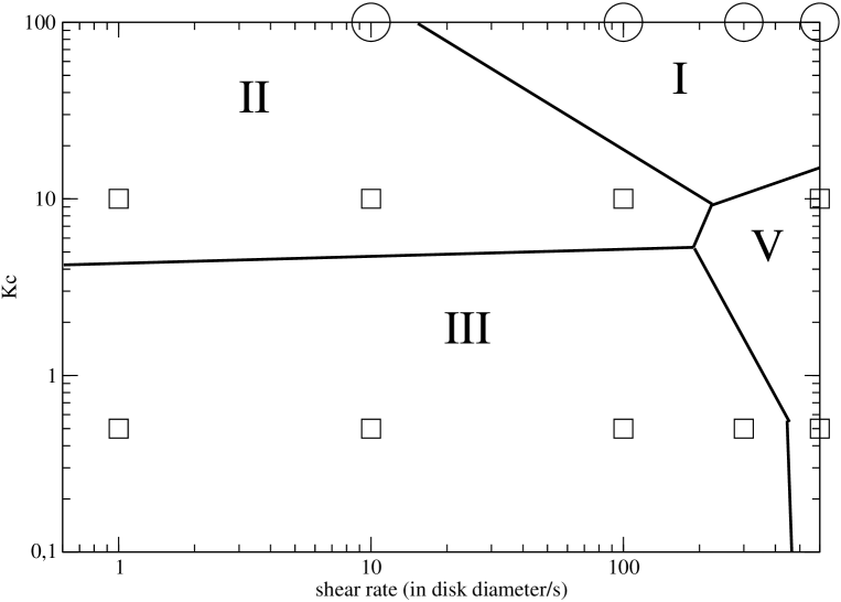
Figure 4: Diagram of the computed shear signal for a shear cell with blades and for cohesive disks as a function of the elastic constant $K_{c}$ ( $g.s^{-2}$) of the cover and of the shear rate (in disk diameter per $s^{-1}$)

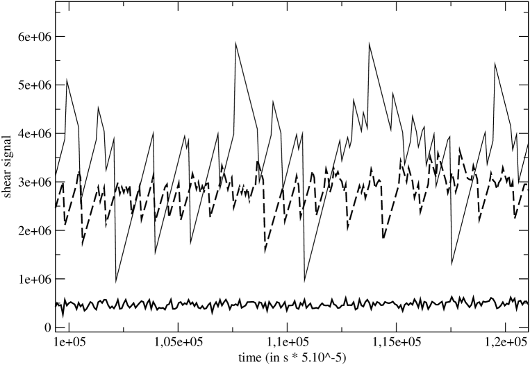
Figure 5: Examples of computed shear signals as a function of time. Shear signal which is irregular in shape (continuous line), regular in shape but irregular in time (long dashed line), non linear in shape (thin continuous line). Experimental examples of similar behaviors may be seen in ref.oliver .

Figure 1 presents the different behaviors of the shear signal for a shear cell without blades and for disks without cohesion as a function of the shear rate and of the elasticity constant of the cover. Figure 2 presents the same feature for disks with cohesion. Figures 3 and 4 correspond to a shear cell with blades for respectively non cohesive and cohesive disks. An example of different stick slip signals is presented in figure 5. The black bold curve corresponds to region II, the long dashed curve corresponds to region IV and the thin continuous curve corresponds to region III.

Let us first analyze the elasticity of the setup and disks leading to the behavior corresponding to region I in fig. 1,2,3 and 4.

Region I is uniquely present when the cover is pulled with an infinite elasticity, i.e. when it slides at a constant rate. The presence of cohesion between the disks does not change this behavior neither the presence of blades on the cover. This characteristic behavior is the one which has been studied in ref. olivi2 . In this previous study, the authors showed that the whole assembly of disks could be replaced by one single spring in the case of cohesive disks. Here, we have the same behavior (presence of a characteristic frequency of the shear signal but irregular signal) even when there is no cohesion between the disks. Straightforwardly, we can say that, as the cohesion has the dimension of a Young modulus, it only modifies the resulting (effective) Young modulus of the disks. Therefore, the assembly of disks behaves as a single spring which is the only source of elasticity in the experiment.

Now, considering region II , let us compare fig. 1,2,3 and 4. In fig. 1, corresponding to a setup with a varying elasticity and disks without cohesion, the shear signal is irregular in time and in shape for all the values of the elasticity of the cover but only for small shear rates. In fig. 2, this behavior disappears for shear rates larger than 0.4$mm.s^{-1}$ for the same values of the elasticity of the cover. In fig. 3 and 4, only elasticities of the cover larger than 10 lead to this behavior, in the case of shear rates smaller than 20$mm.s^{-1}$. We can say that the three (resp. two) origins of elasticities for fig. 2 and 4 (resp. for fig. 1 and 3) lead to an incoherent shear signal which in these cases has no characteristic frequency and is irregular in time. The system in this case is equivalent to 2 or 3 springs in series, with equivalent spring constant. The resulting shear signal is therefore incoherent.

Region III corresponds to shear signals which are smooth but irregular in time. Moreover, the shear signal corresponding to the stick and to the slip stages are curved, showing a non linearity in the elasticity of the experiment. Region III is absent in fig.1 and appears in fig. 2 3 and 4 for small spring constant (equal to 1) of the cover. Here again we can say that the experiment is equivalent to two or three springs in series; but, contrarily to the behavior of the shear signal of region II, the spring constant of the cover is small and becoming dominant in the behavior of the system (we recall that the resulting spring constant of springs in series is the inverse of the sum of inverses of each spring constant).

Region IV corresponds to shear signals which are regular in shape but not regular in time (with no characteristic frequency). As for region III, the system in this case may be modelled by two or three springs in series, the spring with the lowest spring constant is dominant giving the behavior of the resulting shear signal. The difference between the spring constant of the cover and the one or two other spring constants (representing the disks assembly and the cohesion) is smaller than in the case of region III.

In the case of region V, we can always consider that the system is equivalent to two or three springs in series. We can consider that there is a characteristic frequency of the shear signal because the two or three spring constants have each a characteristic frequency close from each other.

As a summary, let us calculate the spring constants of each of the components of the system. The spring constant $K_{c}$ of the cover is an input parameter of the computation. The spring constant $K_{d}$ of the beads without cohesion (dry beads) may be given by:

$$K_{d}=\frac{1}{(\sum_{i=1,n}1/\frac{1}{\sum_{j=1,m}1/K_{b1}})}=\frac{K_{b1}}{mn}$$ (9)

where $K_{b1}$ is the spring constant directly related to the Young modulus $Y$ of one bead. $n$ corresponds to the mean number of disks per vertical line in the shear cell while $m=40$ is the mean horizontal number of disks per horizontal line. This is equivalent to say that we have $n$ equivalent springs in series each of these equivalent springs being one line of $m$ disks in series.

Similarly, the equivalent spring constant $K_{h}$ of cohesive disks (humid disks) may be computed using the same formula but with a value of the equivalent spring constant $K_{b2}$ of each disks modified in order to take account of the cohesion and of the Young modulus which can be considered as springs acting in parallel $K_{b2}=(Y+K)d_{i}$. The equivalent spring constant of the assembly of disks is then approximatively equal to $K_{h}=\frac{K{b2}}{mn}$.

Depending on the geometry of the shear cell, the values of $n$ may vary. Indeed, in a shear cell with blades, only the disks which are below the blades enter the shearing process. For the shear cell without blades, $n=18$ and for the shear cell with blades $n=13$ corresponding to the the number of active disks in the shear process, per vertical line. Therefore, the actual values are for the cover $K_{c}=1,10,\infty g.s^{-2}$,for the shear cell without blades and for disks without cohesion $K_{d}=0.4g.s^{-2}$ and for disks with cohesion $K_{h}=0.415g.s^{-2}$. In the case of the shear cell with blades $K_{d}=0.56g.s^{-2}$ and for disks with cohesion $K_{h}=0.57g.s^{-2}$. The shear signal is regular in shape when $K_{c}$ is of the same order than $K_{d}$ or $K_{h}$ and for large shear rates, like in regions IV and V. Otherwise, the shear signal is irregular in shape.

In ref. olivi , we saw that the position of the spring corresponding to the assembly of disks could be modelled by the following equation:

$$x(t)=\frac{v}{\omega}\sin(\omega t)$$ (10)

where $v$ is the shear rate and $\omega=\sqrt{\frac{K_{e}}{M}}$, with $K_{e}$ the equivalent spring constant of the disks and $M$ the mass of the disks assembly. Here again we may use this equation for the whole system assuming that the equivalent spring constant is $K_{e}=1/(\frac{1}{K_{c}}+\frac{1}{K_{hord}})$ and $M$ is the sum of the mass of the cover and of the disks assembly. Therefore, one may see that if the value of $v$ is much larger than $K_{e}$ the shear signal presents a characteristic frequency like in regions I and V. If the value of $v$ is smaller than $K_{e}$, no characteristic frequency appears like in regions II,III and IV.

Finally, we can say that the shape of the signal and its frequency may be analyzed separately. The shape of the signal depends on the relative values of all components of the system while the frequency of the shear signal depends on the mass, the shear rate and the elasticity of the system.

IV Conclusion

We made a numerical simulations by molecular dynamics of the shearing of twodimensional disks. Depending on the elastic constant of each component of the set up (of the cover, of the disks, and of the cohesion between the disks) and of the shear rate, the resulting simulated shear signal is either regular or irregular in shape, and with or without a characteristic frequency. An analytic analysis allowed us to understand this behavior in the light of the relative values of the elastic constants entering the setup. It appears that we found a regular shear signal only for given values of the elastic constants and of the shear rate.

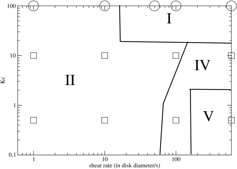
Figure 1: Diagram of the computed shear signal for a shear cell withoud blades and for disks without cohesion as a function of the elastic constant $K_{c}$ ($g.s^{-2}$) of the cover and of the shear rate (in disk diameter per $s^{-1}$)

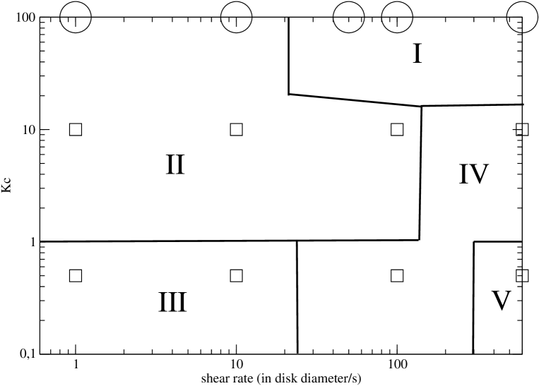
Figure 2: Diagram of the computed shear signal for a shear cell without blades and for cohesive disks as a function of the elastic constant $K_{c}$ ( $g.s^{-2}$) of the cover and of the shear rate (in disk diameter per $s^{-1}$)

References

- (1) C.A.Coulomb, Mémoires de mathématiques et de Physique, Académie Royale des Sciences vol. 7(1773) 343
- (2) F.Bowden, The friction and lubrication of solids, Clarendon Press, Oxford (2001)
- (3) J.H.Dieterich, Trans. Am. Geophys. Union, 51 (1970)
- (4) J.H.Dieterich, Pure and App. Geoph. 116 (1978)
- (5) F.Heslot, T.Baumberger, B.Perrin, B.Caroli and C.Carloi, Phys. Rev. E 49 (1994) 4973
- (6) T.Baumberger, C.Caroli, B.Perrin and O.Ronsin, Phys. Rev. E 51 (1995) 4005
- (7) J.H.Dieterich, J.of Geophysical Res. 84 (1979) 2161
- (8) A.Ruina, J. of Geophysical Res. 88 (1983) 10359
- (9) S.Nasuno, A.Kudrolli and J.P.Gollub, Phys. Rev. Lett. 79 (1997) 949
- (10) S.Nasuno, A.Kudrolli, A.Bak and J.P.Gollub, Phys. Rev. E 58 (1998) 2161
- (11) M.Lubert and A. De Ryck, Phys. Rev. E 63 (2001) 021502
- (12) A. De Ryck, R.Condotta and M.Lubert, Eur. Phys. J. E 11 (2003) 159
- (13) C.Coste, Phys. Rev. E 70 (2004) 051302
- (14) I.Albert, P.Tegzes, R.Albert, J.G.Sampl, A.L.Barabasi, B.Kahng and P.Schiffer, Phys. Rev. E 64 (2001) 1307
- (15) J.Geng and R.P.Behringer, Phys. Rev. E 71 (2005) 011302
- (16) O.Pozo , N.Fraysse and N.Olivi-Tran in Powder and Grains 2005 R.García-Rojo, H.J. Herrmann & S. McNamara, Eds. A.A.Balkema, Rotterdam, 2005
- (17) P.A.Thompson and G.S.Grest, Phys. Rev. Lett. 67 (1991) 1751
- (18) N.Olivi-Tran, O.Pozo and N.Fraysse, J. of Phys. Cond. Matt. 17 (2005) 5677
- (19) G.H. Ristow , Granular Dynamics: a Review about recent Molecular Dynamics Simulations of Granular Materials in Annual Review of Computational Physics, edited by D. Stauffer (World Scientific,1994) Vol. I, p.275
- (20) G.H.Ristow ,Europhys. Lett. 34 (1996) 263
- (21) N.Olivi-Tran ,N. Fraysse ,P. Girard ,M. Ramonda and D. Chatain Eur. Phys. J. B 25 (2002) 217
- (22) N. Olivi-Tran , O. Pozo and N. Fraysse Model. and Simul . in Mat. Sci. and Eng.12 (2004) 671