The quadrupolar phases of the $S=1$ bilinear–biquadratic Heisenberg model on the triangular lattice

Abstract

Using mean-field theory, exact diagonalizations and $SU({3})$ flavour theory, we have precisely mapped out the phase diagram of the $S=1$ bilinear–biquadratic Heisenberg model on the triangular lattice in a magnetic field, with emphasis on the quadrupolar phases and their excitations. In particular, we show that ferroquadrupolar order can coexist with short-range helical magnetic order, and that the antiferroquadrupolar phase is characterized by a remarkable 2/3 magnetization plateau, in which one site per triangle retains quadrupolar order while the other two are polarized along the field. Implications for actual $S=1$ magnets are discussed.

When discussing quantum magnets, it is useful to classify models according to whether or not the ground state breaks the $SU({2})$ symmetry. While simple examples of both cases are well known (long-range magnetic order for broken $SU({2})$ symmetry, spin ladders for non-broken $SU({2})$ symmetry), a lot of activity is currently devoted to the problem of identifying more exotic ground states of either type. In the context of non-broken $SU({2})$ symmetry, the attention is currently focused on the search for Resonating Valence Bond ground states in frustrated quantum magnets (for a review see claire ).

Regarding $SU({2})$ broken ground states, the existence of nematic order spin_nematics is well documented in a number of models, but its identification is faced with two difficulties: First of all, these models usually require four-spin exchange ring or biquadratic spin interactions harada that are rather large for Mott insulators FM . Besides, nematic order does not give rise to magnetic Bragg peaks, and there is a need for simple criteria that could help identifying nematic order experimentally.

In that respect, the recent investigation of NiGa₂S₄ nigas , and the subsequent proposal by Tsunetsugu and Arikawa tsune that some kind of antiferroquadrupolar (AFQ) order might be at the origin of the anomalous properties of that system, are very stimulating. They have investigated the AFQ phase of the $S=1$ Heisenberg model with bilinear and biquadratic exchange on the triangular lattice, defined by the Hamiltonian:

$$\mathcal{H}=J\sum_{\langle i,j\rangle}\left[\cos\vartheta\ {\bf S}_{i}\cdot{\bf S}_{j}+\sin\vartheta\left({\bf S}_{i}\cdot{\bf S}_{j}\right)^{2}\right]-h\sum_{i}S_{i}^{z}\;.$$ (1)

Using a bosonic description of the excitations, they have investigated the zero-field case and shown in particular that: 1) The magnetic structure factor has a maximum but no Bragg peak; 2) The susceptibility does not vanish at zero temperature; 3) The specific heat has the characteristic $T^{2}$ behaviour of 2D systems with broken $SU({2})$ symmetry. These features agree qualitatively with the properties of NiGa₂S₄, but several points remain to be addressed. In particular, unlike the AFQ phase of the Heisenberg model studied in Ref. tsune, , the short-range magnetic fluctuations are incommensurate in NiGa₂S₄. So the actual magnetic model describing NiGa₂S₄ remains to be worked out. Maybe more importantly, a more direct identification of quadrupolar order as being at the origin of its properties would be welcome.

In the present paper, we address these points in the context of a thorough investigation of the $S=1$ bilinear-biquadratic Heisenberg model on the triangular lattice, Eq. (1). We put special emphasis on the quadrupolar phases and on the effect of a magnetic field.

Quadrupolar operators and states:

To discuss quadrupolar (QP) order, it is useful to introduce the QP operator ${\bf Q}_{i}$ of components $(S_{i}^{x})^{2}-(S_{i}^{y})^{2}$, $(2(S_{i}^{z})^{2}-(S_{i}^{x})^{2}-(S_{i}^{y})^{2})/\sqrt{3}$, $S_{i}^{x}S_{i}^{y}+S_{i}^{y}S_{i}^{x}$, $S_{i}^{y}S_{i}^{z}+S_{i}^{z}S_{i}^{y}$, and $S_{i}^{x}S_{i}^{z}+S_{i}^{z}S_{i}^{x}$. In the finite Hilbert space of $S=1$, the biquadratic term can also be expressed by quadrupolar operators, and the Hamiltonian can be rewritten as

$$\mathcal{H}=\sum_{\langle i,j\rangle}\left[\left(J_{1}-\frac{J_{2}}{2}\right){\bf S}_{i}\cdot{\bf S}_{j}+\frac{J_{2}}{2}{\bf Q}_{i}\cdot{\bf Q}_{j}+\frac{4}{3}J_{2}\right]$$ (2)

with $J_{1}=J\cos\vartheta$ and $J_{2}=J\sin\vartheta$. Since ${\bf Q}_{i}\cdot{\bf Q}_{j}+{\bf S}_{i}\cdot{\bf S}_{j}=-2\mathcal{P}_{i,j}-2/3$, and since the permutation operator $\mathcal{P}_{i,j}$ has $SU({3})$ symmetry for spin 1, the Hamiltonian is $SU({3})$ symmetric for $J_{1}=J_{2}$ ($\vartheta=\pi/4$ and $-3\pi/4$). It turns out to be convenient to choose the following time–reversal invariant basis of the $SU({3})$ fundamental representation:

$$|x\rangle=\frac{i|1\rangle-i|\bar{1}\rangle}{\sqrt{2}};\quad|y\rangle=\frac{|1\rangle+|\bar{1}\rangle}{\sqrt{2}};\quad|z\rangle=-i|0\rangle\,.$$ (3)

Quadupolar spin-states are then defined as linear combinations with real amplitudes $d_{\nu}$ (such that $|{\bf d}|=1$)

$$|Q({\bf d})\rangle=d_{x}|x\rangle+d_{y}|y\rangle+d_{z}|z\rangle$$ (4)

$|Q({\bf d})\rangle$ is time–reversal invariant, which implies that $\langle Q({\bf d})|{\bf S}|Q({\bf d})\rangle=0$, and it is a zero eigenvalue eigenstate of the operator $\left({\bf d}\cdot{\bf S}\right)^{2}$. It describes a state where the spin fluctuates mostly in the directions perpendicular to the vector ${\bf d}$, referred to as the director, which nicely illustrates the very heart of a spin nematic state: it has no magnetic moment, but nevertheless breaks $SU({2})$ symmetry due to the presence of anisotropic spin fluctuations.

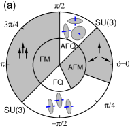
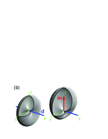
Figure 1: (color online) (a) Zero-field phase diagram. The inner circle is the variational result, the outer circle the exact–diagonalization one. The magnetic phases are shaded in gray. (b) Probabilities of spin fluctuations $|\langle S(\hat{\bf n})|\psi\rangle|^{2}$ in the pure state $\psi=|y\rangle$ (left) and in a state with finite magnetization (right). $|S(\hat{\bf n})\rangle$ is the coherent spin state pointing in direction $\hat{\bf n}$.

Zero-field phase diagram:

First, we construct the variational (mean-field) phase diagram in the variational sub-space of site–factorized wave functions of the form $\prod_{j}|Q({\bf d}_{j})\rangle$, allowing complex ${\bf d}_{j}$’s ivanov03 , and assuming 3–sublattice long–range order. Without magnetic field, we get four phases (Fig. 1). Adjacent to the usual ferromagnetic (FM) phase, which is stabilized for $\pi/2<\vartheta<5\pi/4$, we find two QP phases. The expectation value of ${\bf Q}_{i}\cdot{\bf Q}_{j}$ in the site–factorized wave function subspace is

$$\langle{\bf Q}_{i}\cdot{\bf Q}_{j}\rangle=2|{\bf d}_{i}\cdot{\bf d}_{j}|^{2}-2/3;\quad i\neq j\;.$$ (5)

Since it induces a negative QP exchange, a negative biquadratic exchange tends to drive the directors collinear, leading to a stabilization of the ferroquadrupolar (FQ) state for $-3\pi/4<\vartheta<\Theta^{MF}_{c}$ with $\Theta^{MF}_{c}=\arctan(-2)\approx-0.35\pi$. On the other hand, a positive biquadratic term induces a positive QP exchange, which is minimized with mutually perpendicular directors. On the triangular lattice, this is not frustrating since all bonds can be satisfied simultaneously by adopting a 3-sublattice configuration with e.g. directors pointing in the $x$, $y$ and $z$ directions respectively, a phase that can be called antiferroquadrupolar (AFQ). This is realized between the $SU({3})$ point and the FM phase ($\pi/4<\vartheta<\pi/2$).

For $\Theta^{MF}_{c}<\vartheta<\pi/4$, we get the standard 3–sublattice 120^∘–antiferromagnetic (AFM) phase, but with a peculiarity: the spin length depends on $J_{2}/J_{1}$. It is maximal ($|\langle{\bf S}\rangle|=1$) for $J_{2}=0$ and vanishes continuously as $|\langle S\rangle|\propto\sqrt{2J_{1}-|J_{2}|}$ at the FQ boundary, where the trial wave function becomes a QP state with the director perpendicular to the plane of the spins. Approaching the $SU({3})$ point, $|\langle{\bf S}\rangle|\rightarrow\sqrt{8}/3$, and the wave functions on the three sublattices become orthogonal. Actually, at this highly symmetric point any orthogonal set of wave functions is a good variational ground state. It includes the AFQ state as well, which is connected to the AFM state by a global $SU({3})$ rotation.

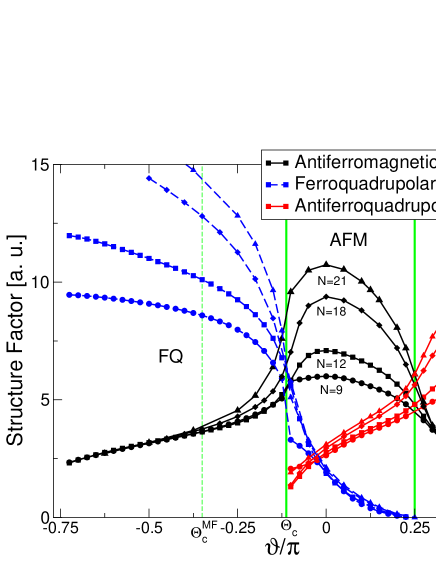
Figure 2: (color online) Spin and quadrupolar structure factors at the $\Gamma$ and K points for different finite clusters. The system sizes are labeled by the symbol type.

Next, we have performed finite–size exact diagonalization calculations on samples with up to 21 sites. In Fig. 2, we show the size dependence of the correlation functions associated with the FQ, AFM and AFQ order. More specifically we determine the structure factors $\sum_{j}\exp[i\mathbf{k}\cdot\mathbf{r}_{j}]\langle\mathcal{C}_{0}\cdot\mathcal{C}_{j}\rangle$, where $\mathcal{C}_{j}$ stands for the spin or quadrupolar operator at site $j$ and $\mathbf{k}$ is the $\Gamma$ or $K$ point in the Brillouin–zone for the ferro or antiferro phases, respectively. As can be clearly seen, the $SU({3})$ point separates the AFM and AFQ phases, and the $\vartheta$ dependence of the structure factors in the AFQ range is reminiscent of that reported in the 1D model andreas_1D . The phase boundary between the FQ and AFM phases is, on the other hand, strongly renormalized from the mean-field value $\Theta^{MF}_{c}\approx-0.35\pi$ to about $\Theta_{c}\approx-0.11\pi$ ($J_{2}\approx-0.4J_{1}$) note_phaseboundary . We have also verified the presence of the appropriate Anderson towers of states in the energy spectrum for the FQ, AFM, $SU({3})$ AF, and AFQ phase longpaper . Let us emphasize that we found no indication of disordered or liquid phases in that model.

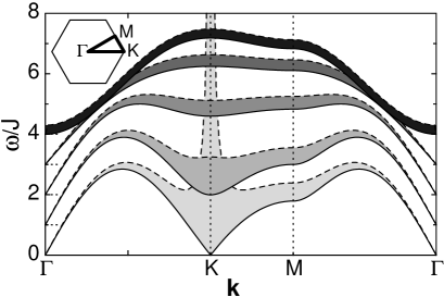
Figure 3: Spin correlation function $S({\bf k},\omega)$ from flavor-wave calculation for $\vartheta=-3\pi/4$, $-5\pi/8$, $-\pi/2$, $-3\pi/8$, and $\Theta^{MF}_{c}$ from top to bottom (shifted by J) in the FQ phase. The dispersion $\omega(q)$ is the solid curve, the matrix element is the dashed line measured from the solid line. Left upper corner: the Brillouin zone.

Quadrupole waves:

Since the usual spin–wave theory is not adequate to describe the excitations of QP phases, we use the flavour-wave theory of papanicolaou84 . We associate 3 Schwinger–bosons $a_{\nu}$ to the states of Eq. (3) and enlarge the fundamental representation on a site to a fully symmetric $SU({3})$ Young-diagram consisting of an $M$ box long row. The spin operators are expressed as $S^{\alpha}(j)=-i\epsilon_{\alpha\beta\gamma}a_{\beta}^{\dagger}(j)a_{\gamma}^{\phantom{\dagger}}(j)$. Condensing the bosons associated with the ordering then leads to a Holstein-Primakoff transformation. This approach is equivalent to the bosonic description of the AFQ phase in tsune , so we will concentrate on FQ phase. To describe a state with all directors pointing in the $y$ direction, we let the $y$ bosons condense and replace $a_{y}^{\dagger}$ and $a_{y}^{\phantom{\dagger}}$ by $(M-a_{x}^{\dagger}a_{x}^{\phantom{\dagger}}-a_{z}^{\dagger}a_{z}^{\phantom{\dagger}})^{1/2}$. A $1/M$ expansion up to quadratic order in the Holstein-Primakoff bosons $a_{x}$ and $a_{z}$ followed by a standard Bogoliubov transformation leads to:

$$\mathcal{H}=\sum_{\nu=x,z}\sum_{\bf k}\omega_{\nu}({\bf k})\left[\alpha_{\nu}^{\dagger}({\bf k})\alpha_{\nu}({\bf k})+1/2\right]\,,$$ (6)

with $\omega_{\nu}({\bf k})=\sqrt{A^{2}_{\nu}({\bf k})-B^{2}_{\nu}({\bf k})}$, $A_{\nu}({\bf k})=3(J_{1}\gamma({\bf k})-J_{2})$, $B_{\nu}({\bf k})=3(J_{2}-J_{1})\gamma({\bf k})$, and $\gamma({\bf k})=\sum_{{\bf r}}\exp(i{\bf r}\cdot{\bf k})/6$, where ${\bf r}$ spans the 6 neighbours of a site. We get two branches of quadrupole waves associated to $a_{x}$ and $a_{z}$. In zero field, they are degenerate throughout the entire Brillouin zone.

The imaginary part of the spin-spin correlation function (shown in Fig. 3) is given by:

$$S^{xx}({\bf k},\omega)=\frac{A_{z}({\bf k})+B_{z}({\bf k})}{\omega_{z}({\bf k})}\delta(\omega-\omega_{z}({\bf k}))\;.$$ (7)

The $\nu=z$ branch contributes to $S^{xx}({\bf k},\omega)$ – the spin fluctuations are perpendicular to both the director $y$ and the direction of the QP excitation $z$. Correspondingly, the $\nu=x$ branch contributes to $S^{zz}({\bf k},\omega)$, which is equal to $S^{xx}({\bf k},\omega)$. $S^{yy}({\bf k},\omega)=0$ (it appears in higher order in $1/M$). Close to the $\Gamma$ point, both the dispersion of the flavor-wave and the correlation function are linear in $k$: $\omega_{\nu}({\bf k})=vk$ and $S^{xx}({\bf k})=S^{zz}({\bf k})=\chi vk$, where $\chi=1/[6(J_{1}-J_{2})]$ is the mean–field susceptibility and $v=\sqrt{9J_{2}(J_{2}-J_{1})/2}$. As we approach the boundary to the AFM phase, $\omega_{\nu}({\bf k})$ softens and the spin structure factor diverges at the $K$ point of the Brillouin zone as $S({\bf k})\propto\xi(1+\xi^{2}|{\bf k}-{\bf k}_{K}|^{2})^{-1/2}$, where the correlation length $\xi=1/\sqrt{10(\Theta_{c}^{MF}-\vartheta)}$ is associated with the short range easy–plane 120^∘ AFM order. So FQ order can coexist with non-ferromagnetic short-range correlations, a result to keep in mind when comparing with experiments.

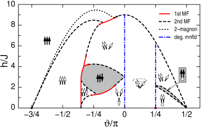
Figure 4: (color online) Magnetic phase diagram. Solid (dashed) lines denote 1st (2nd) order phase boundaries in the variational approach. The dotted line shows the exact boundary of the FQ phase (two magnon bound state formation, see Ref.longpaper ). Along the dashed–dotted lines the variational solution is highly degenerate. The plateaux are shaded in gray. Filled arrows represent fully polarized magnetic moments, empty arrows partially polarized ones.

Finite magnetic field:

In this case, the variational phase diagram is surprisingly rich, as shown in Fig. 4.

For $0<\vartheta<\pi/4$, the 3-sublattice AFM order gives rise to the chiral umbrella configuration up to full polarization. However, for negative $J_{2}$, a $m=1/3$ plateau occurs with up-up-down configuration, reminiscent of the plateau reported for the $S=1/2$ case Honecker . Interestingly enough, this magnetic configuration is also realized below the plateau close to the FQ phase. Above the plateau, the spin configuration is coplanar (see Fig. 4).

In the FQ phase, the directors turn perpendicular to the magnetic field ivanov03 , and the QP state is given by:

$$|\psi_{j}\rangle=\cos\frac{\mu}{2}|Q(d_{x},d_{y},0)\rangle+i\sin\frac{\mu}{2}|Q(-d_{y},d_{x},0)\rangle\;.$$ (8)

It develops a magnetic moment $m=\langle S^{z}\rangle=\sin\mu$ parallel to the magnetic field by shifting the center of the fluctuations [c.f. Fig. 1(b)] . The magnetization grows linearly with the magnetic field as $m=h/[6(J_{1}-J_{2})]$. One of the two degenerate gapless modes acquires a gap proportional to the field, while the other one remains gapless – it is the Goldstone mode associated with the rotation of the director in the $xy$ plane longpaper .

The most surprising feature of the phase diagram is the magnetization plateau at $m=2/3$ that occurs starting from the AFQ phase ($\pi/4<\vartheta<\pi/2$) tsunem2o3 . This plateau is of mixed character: It is a $|110\rangle$ state, where $|1\rangle$ is magnetic and $|0\rangle$ QP. It is stable between $h=3J_{1}$ and $3(4J_{1}-3J_{2}+\sqrt{9J_{2}^{2}-8J_{1}J_{2}})/2$ according to the variational calculation, a result confirmed by exact diagonalizations of the magnetization for systems with up to 27 sites: There is indeed clear evidence of a plateau at 2/3, and the overall magnetization curve is in good agreement with the mean-field result, as shown in Fig. 5. Note that the occurrence of a plateau at 2/3 without a plateau at 1/3 is truly remarkable. Indeed, this is very unlikely to occur for purely magnetic states since the 2/3 plateau would correspond to a higher commensurability (5 up, 1 down in the simplest scenario) than the 1/3 one. This plateau can be considered as a characteristic of AFQ order. Below the $m=2/3$ plateau, for $\pi/4<\vartheta<\pi/2$ and $h<3\cos\vartheta$ the variational ground state is the deformed QP state of Eq. (8), with two perpendicular directors in the $xy$ plane, while on the third sublattice the QP state is $|0\rangle$. The magnetization is given by $m=2h/(9J_{1})$.

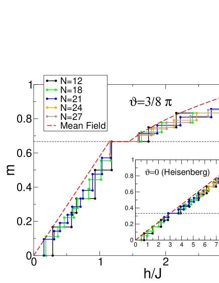
Figure 5: (color online) Magnetization curves obtained by exact diagonalization for $\vartheta=3\pi/8$, where the presence of a plateau at $m=2/3$ is confirmed. The inset shows a magnetization curve at the Heisenberg point with a small plateau stabilized at $m=1/3$.

Discussion:

Let us put these results in experimental perspective. The occurrence of FQ order for negative biquadratic exchange makes it a more likely candidate a priori. Indeed, a mechanism based on orbital quasi-degeneracy has been shown to naturally lead to a negative biquadratic coupling orbitalbiquadratic . In contrast, mechanisms leading to a large positive biquadratic coupling remain to be found. Otherwise, the FQ and AFQ have a lot in common, in particular gapless modes, maxima but no Bragg peaks in the magnetic structure factor, a $T^{2}$ specific heat and a linear magnetization at low field. Let us emphasize that the location of the maxima depends primarily on the bilinear exchange (sign, topology, range,…) and is not directly related to that of the gapless modes, which depends on the type of QP order, hence on the sign of the biquadratic exchange. The main difference is the presence of a remarkable magnetization $m=2/3$ plateau in the AFQ phase. In addition, the removal of one of the gapless modes of the FQ state in a field should be visible in the low temperature specific heat. Regarding NiGa₂S₄, it will be interesting to include further neighbor bilinear interactions into the present model to see if a QP phase with dominant incommensurate fluctuations can be stabilized. The properties of the corresponding phase are expected to depend strongly on the sign of the biquadratic coupling, and the results of the present paper should help in identifying such a phase.

- (1) G. Misguich and C. Lhuillier, cond-mat/0310405. published in ”Frustrated spin systems”, H. T. Diep, ed., WorldScientific, (2005).
- (2) A.F. Andreev and I.A. Grishchuk, Zh. Eksp. Teor. Fiz. 87, 467 (1984) [Sov. Phys. JETP 60, 267 (1984)]; A. Chubukov, J. Phys. Condens. Matter 2 1593 (1990).
- (3) A. Läuchli, J.C. Domenge, C. Lhuillier, P. Sindzingre, and M. Troyer, Phys. Rev. Lett. 95, 137206 (2005).
- (4) K. Harada and N. Kawashima, Phys. Rev. B 65, 052403 (2002).
- (5) Note however that a small nematic phase has been recently reported in a pure Heisenberg model with competing ferromagnetic and antiferromagnetic exchanges (N. Shannon, T. Momoi, and P. Sindzingre, Phys. Rev. Lett. 96, 027213 (2006)).
- (6) S. Nakatsuji et al., Science 309, 1697 (2005).
- (7) H. Tsunetsugu and M. Arikawa, J. Phys. Soc. Jap. 75, 083701 (2006).
- (8) B. A. Ivanov and A. K. Kolezhuk, Phys. Rev. B 68, 052401 (2003).
- (9) A. Läuchli, G. Schmid, S. Trebst, cond-mat/0311082.
- (10) While we cannot exclude on the basis of the present results that long-wave length fluctuations stabilize the AFM order below that critical value, the presence of a level crossing at this value of in the 9 and 21-site clusters with no significant size dependence gives further support to this identification of .
- (11) A. Läuchli, F. Mila, K. Penc, unpublished.
- (12) N. Papanicolaou, Nucl. Phys. B 240, 281 (1984); A. Joshi, M. Ma, F. Mila, D. N. Shi, and F. C. Zhang, Phys. Rev. B 60, 6584 (1999).
- (13) A. Honecker, J. Schulenburg and J. Richter, J. Phys.: Condens. Matter 16, S749-S758 (2004); H. Nishimori and S. Miyashita J. Phys. Soc. Japan 55, 4448 (1986).
- (14) This plateau has been found independently by Tsunetsugu and Arikawa (H. Tsunetsugu, private communication).
- (15) F. Mila and F.C. Zhang, Eur. Phys. J. B 16, 7 (2000).