Variational ground states of 2D antiferromagnets in the valence bond basis

Abstract

We study a variational wave function for the ground state of the two-dimensional $S=1/2$ Heisenberg antiferromagnet in the valence bond basis. The expansion coefficients are products of amplitudes $h(x,y)$ for valence bonds connecting spins separated by $(x,y)$ lattice spacings. In contrast to previous studies, in which a functional form for $h(x,y)$ was assumed, we here optimize all the amplitudes for lattices with up to $32\times 32$ spins. We use two different schemes for optimizing the amplitudes; a Newton/conjugate-gradient method and a stochastic method which requires only the signs of the first derivatives of the energy. The latter method performs significantly better. The energy for large systems deviates by only $\approx 0.06\%$ from its exact value (calculated using unbiased quantum Monte Carlo simulations). The spin correlations are also well reproduced, falling $\approx 2\%$ below the exact ones at long distances. The amplitudes $h(r)$ for valence bonds of long length $r$ decay as $r^{-3}$. We also discuss some results for small frustrated lattices.

I Introduction

The valence bond (VB) basis for singlet states of quantum spin systems was first discussed by Rumer rum32 and Pauling pau33 in the 1930s and was shortly thereafter applied in Heisenberg spin chain calculations by Hulthén.hul38 For a systems of $N$ $S=1/2$ spins the overcomplete and non-orthogonal VB basis consists of states that are products of $N/2$ spin pairs forming singlets. In the most general case the members of a singlet can be separated by an arbitrary distance, but it is often convenient to consider a restricted set of configurations with only bonds connecting two different groups of sites, e.g., the two sublattices of a bipartite lattice. Such a restricted VB basis is still overcomplete and any singlet state can be expanded in it. Any restriction on the maximum length of the bonds will render the basis incomplete, however.

After Anderson’s proposal in 1987 of a resonating-valence-bond (RVB) state fez74 as a natural starting point for understanding high-temperature superconductivity in the cuprates,and87 variational VB states were investigated for both doped and undoped antiferromagnets.lia88 ; gros ; capriotti ; bon91 ; fano ; havilio1 ; havilio2 ; poilblanc The RVB spin liquid mechanism is based on states dominated by short valence bonds, which in the extreme case have been argued to correspond closely to the quantum dimer model.kiv87 It was early on established, however, that the ground state of the two-dimensional (2D) Heisenberg model with nearest-neighbor interactions, which has a Néel ordered ground state and describes very well the undoped cuprates,chn ; man91 actually requires an algebraic, not exponential, decay of the bond-length probability.lia88

Some attempts were made to use the VB basis as a framework for numerical calculations, isk87 ; koh88 ; tan88 ; sut88 ; lia90 ; fano but, with very few exceptions,san99 these efforts were not pursued further in large scale quantum Monte Carlo calculations (QMC). However, it was recently pointed out that there are previously unnoticed advantages of carrying out ground state projector QMC calculations in the VB basis, including a natural way to access excitations in the triplet sector.san05 ; beachvbs ; beachinprep Such a scheme has already been applied to 2D and 3D models with valence bond solid ground states.vb2d ; vb3d

It may also be worthwhile to pursue further variational schemes in the VB basis, especially exploring possibilities to study frustrated systems this way. In this paper we report a bench-mark variational calculation going beyond previous VB variational studies lia88 of the 2D Heisenberg model. Instead of assuming a functional form for the bond-length amplitudes and optimizing a few parameters, we optimize all individual amplitudes in order to definitely establish the properties of this kind of wave function and its ability to reproduce the ground state of the 2D Heisenberg model. We also report some preliminary studies of a frustrated system.

For the standard 2D Heisenberg model with nearest-neighbor coupling $J$, the energy of our best optimized wave function deviates by only $\Delta E/J\approx 0.06\%$ from the exact ground state energy for system with up to $32\times 32$ spins. The size dependence of $\Delta E$ shows that this accuracy should persist in the thermodynamic limit. The error is only half that of the best wave functions found in the previous variational QMC study.lia88 The spin-spin correlations are also remarkably well reproduced; they are approximately $2\%$ smaller than the exact values at long distances, corresponding to an $\approx 1\%$ underestimation of the sublattice magnetization. We find that the asymptotic form of the amplitudes for bonds of length $r$ is $h(r)\sim r^{-3}$, which has also been found recently in a mean-field calculation. beachmeanfield We also compare the variational wave function with the exact ground state in the case of a $4\times 4$ lattice, and find that the overlap is $\approx 0.9998$. Extending the $4\times 4$ calculation to a frustrated system, the J₁–J₂ model, we find that the quality of the amplitude-product wave function deteriorates as the frustration is increased but the overlap remains above $0.996$ even for $J_{2}/J_{1}$ as high as $0.4$.

In Sec. II we define the variational VB wave function. Technical details of the QMC based optimization methods that we have used to minimize the energy are presented in Sec. III. We discuss both a standard Newton method and a stochastic scheme, which requires only the first derivatives of the energy. The latter method performs significantly better for large lattices. Results for the energy and spin correlations in the standard non-frustrated Heisenberg model are discussed in Sec. IV. Results for energies and overlaps for the $4\times 4$ frustrated lattice are discussed in Sec. V. In Sec. VI we conclude with a brief summary and discussion of the methods and results.

II Model and wave function

We study the standard $S=1/2$ Heisenberg model;

$$H=J\sum_{\langle i,j\rangle}{\bf S}_{i}\cdot{\bf S}_{j},$$ (1)

where $\langle i,j\rangle$ denotes nearest-neighbor sites on a 2D square lattice and $J>0$. The basic properties of this model have been known for a long time,man91 and ground state parameters such as the sublattice magnetization, the energy, and the spin stiffness have been extracted to high precision in many QMC studies.lia90 ; qmc2d ; san97 Here our aim is to investigate how well a simple variational wave function can reproduce the true ground state.

The general form of a VB wave function for $N$ $S=1/2$ spins is

$$|\Psi\rangle = \sum_{k}f_{k}|(a_{1}^{k},b_{1}^{k})\cdots(a_{N/2}^{k},b_{N/2}^{k})\rangle$$ (2)

$$= \sum_{k}f_{k}\mid V_{k}\rangle,$$ (3)

where $(a_{i}^{k},b_{i}^{k})$ represents a singlet formed by the spins at sites $a$ and $b$ in VB configuration $k$;

$$(a,b)=\frac{1}{\sqrt{2}}(\uparrow_{a}\downarrow_{b}-\downarrow_{a}\uparrow_{b}).$$ (4)

The notation $|V_{k}\rangle$ has been introduced in (3) for convenience. In the most general case, the VB configurations $V_{k}$ include all the possible pairings of the $N$ spins into $N/2$ valence bonds. A more restricted, but still massively overcomplete basis is obtained by first dividing the sites into two groups, $A$ and $B$, which in the case of a bipartite lattice naturally correspond to the two sublattices. Here we will use such a restricted VB basis and always (also when considering the frustrated case later on) take $A$ and $B$ to refer to the sublattices of the square lattice. We fix the “direction” of the singlet in (4) by always taking the first index in $(a,b)$ from $A$ and the second one from $B$. With this convention one can show that all the expansion coefficients $f_{k}$ [where $k=1,\ldots,(N/2)!$] in Eq. (3) can be taken positive. This corresponds to the Marshall sign rule for a non-frustrated system in the basis of eigenstates of the $S^{z}_{i}$ operators.lia88 ; sut88

We consider expansion coefficients of the amplitude-product form previously introduced and studied by Liang, Doucot and Anderson;lia88

$$f_{k}=\prod_{i=1}^{N/2}\tilde{h}(a_{i}^{k},b_{i}^{k})=\prod_{i=1}^{N/2}h(x_{i}^{k},y_{i}^{k}),$$ (5)

where $x_{i}$ and $y_{i}$ are the $x$ and $y$ separations (number of lattice constants) between sites $a_{i},b_{i}$, which are connected by valence bond $i$. Considering the lattice symmetries (we use periodic boundary conditions), there are hence $\approx N/16$ independent amplitudes $h(x,y)$ to optimize. In the previous study,lia88 only a few short-length amplitudes were optimized and beyond these an asymptotic form depending only on the length $r$ of the bond was assumed.manhattan With a power-law form, $h(x,y)\sim r^{-p}$, it was found that long-range Neel order requires $p<5$. The best variational energy was obtained with $p=4$, giving a deviation $\Delta E/J\approx 0.0008$ (or $\approx 0.12\%$) from the exact ground state energy (the thermodynamic-limit value of which is san97 $\approx 0.69944$ per site).

We here optimize all $h(x,y)$ using two different methods: A standard Newton method (combined with a conjugate gradient method—the Fletcher Reeves methodvar ), and a stochastic method that we have developed which requires only the signs of the first derivatives.

III Optimization methods

We now discuss the technical details of these calculations. To optimize the energy using a Monte Carlo based scheme, we write its expectation value as

$$E=\langle\Psi|H|\Psi\rangle=\frac{\sum_{kl}f_{k}f_{l}\langle V_{k}|V_{l}\rangle\frac{\langle V_{k}|H|V_{l}\rangle}{\langle V_{k}|V_{l}\rangle}}{\sum_{kl}f_{k}f_{l}\langle V_{k}|V_{l}\rangle},$$ (6)

where on the right-hand side we have taken into account the fact that we do not normalize the wave-function coefficients, i.e., the amplitudes in Eq. (5) are only determined up to an over-all factor. The overlap $\langle V_{k}|V_{l}\rangle$ between two VB states is related to the loops forming when the two bond configurations are superimposed; $\langle V_{k}|V_{l}\rangle=2^{N_{l}-N/2}$, where $N_{l}$ is the number of loops.lia88 ; sut88 Matrix elements of ${\bf S}_{i}\cdot{\bf S}_{j}$ are also easy to evaluate in terms of the loop structure. If $i$ and $j$ belong to the same loop, then $\langle V_{k}|{\bf S}_{i}\cdot{\bf S}_{j}|V_{l}\rangle/\langle V_{k}|V_{l}\rangle$ $=\pm 3/4$ ($+$ for $i,j$ on the same sublattice and $-$ else), and else the matrix element vanishes.lia88 ; sut88 Recently more complicated matrix elements have also been related to the loop structure.beachvbs

For a given set of amplitudes $h(x,y)$, we evaluate the energy using the Metropolis Monte Carlo algorithm described in Ref. lia88, . An elementary update of the bond configuration amounts to choosing two next-nearest-neighbor sites $a,c$ (or in principle any $a,c$ in the same sublattice, but the acceptance rate decreases with increasing distance between the sites), and reconfiguring the bonds $(a,b),(c,d)$ to which they are connected, according to $(a,b)(c,d)\to(a,d)(c,b)$ (where the order of the labels here correspond to both sites $a$ and $c$ being in sublattice A). The Metropolis acceptance probability $P$ for such an update is very easy to calculate in terms of amplitude ratios and the change in the number of loops, $\Delta N_{l}$, in the overlap graph;

$$P={\rm min}\left[\frac{h(x_{ad},y_{ad})h(x_{cb},y_{cb})}{h(x_{ab},y_{ab})h(x_{cd},y_{cd})}2^{\Delta N_{l}},1\right].$$ (7)

III.1 Newton Conjugate Gradient Method

For the optimization we also need derivatives of the energy with respect to the amplitudes. The Newton method requires first and second derivatives. Moving in a certain direction ${\bf\hat{g}}$ in amplitude space, the amplitude vector ${\bf h_{n}}$ is updated from iteration $n$ to $n+1$ according to

$${\bf h}_{n+1}={\bf h}_{n}-\frac{E_{g}^{\prime}({\bf h}_{n})}{E_{g}^{\prime\prime}({\bf h}_{n})}{\bf\hat{g}},$$ (8)

where $E^{\prime}_{g}$ and $E^{\prime\prime}_{g}$ are the first and second derivatives of the energy along the ${\bf\hat{g}}$ direction. They are calculated from the derivatives with respect to the amplitudes $h(x,y)$, which are evaluated during the sampling of VB configurations. Writing the energy expectation value as

$$\langle E\rangle=\frac{\sum_{p}W_{p}E_{p}}{\sum_{p}W_{p}},~{}~{}~{}W_{p}=\prod_{x,y}h(x,y)^{n_{xy}},$$ (9)

where $n_{xy}$ is the total number of VBs of size $(x,y)$ in the VB configurations $V_{k}$ and $V_{l}$, the Monte Carlo estimator for the first derivative is

$$\frac{\partial\langle E\rangle}{\partial h_{a}}=\left\langle\frac{n_{a}}{h_{a}}E\right\rangle-\left\langle\frac{n_{a}}{h_{a}}\right\rangle\left\langle E\right\rangle.$$ (10)

Here, to simplify the notation, we use $a$ as a collective index for $(x,y)$. The second derivatives—the elements of the Hessian matrix—are:

$$\frac{\partial^{2}\langle E\rangle}{\partial h_{a}^{2}} = \frac{1}{h_{a}^{2}}\Bigl{(}\langle n_{a}^{2}E\rangle-\langle n_{a}^{2}\rangle\langle E\rangle-\langle n_{a}E\rangle+\langle n_{a}\rangle\langle E\rangle$$ (11)

$$+2\langle n_{a}\rangle^{2}\langle E\rangle-2\langle n_{a}\rangle\langle n_{a}E\rangle\Bigr{)},$$

$$\frac{\partial^{2}\langle E\rangle}{\partial h_{a}h_{b}} = \frac{1}{h_{a}h_{b}}\Bigl{(}\langle n_{a}n_{b}E\rangle-\langle n_{a}n_{b}\rangle\langle E\rangle+2\langle n_{a}\rangle\langle n_{b}\rangle\langle E\rangle$$ (12)

$$-\langle n_{a}\rangle\langle n_{b}E\rangle-\langle n_{b}\rangle\langle n_{a}E\rangle\Bigr{)}.$$

Since we have many amplitudes $h(x,y)$ to optimize, we choose our optimization direction by the conjugate gradient method. The first direction is the gradient direction. In subsequent steps we choose the direction conjugate to the former one, satisfying the relation

$${\bf h}_{n+1}\cdot{\bf A}\cdot{\bf h}_{n}={\bf 0},$$ (13)

where ${\bf A}$ is the Hessian matrix. In practice, we have found that the number of line optimizations required for energy convergence is of the same order as total number of different amplitudes. Since the optimization is based on quantities obtained using a stochastic scheme, the final results of course have statistical errors.

We have $\propto N^{2}$ different second derivatives and hence computing all of them requires a significant computational effort. Their statistical fluctuations are also relatively large for large lattices. We have also used a minimization method requiring only the first derivatives, where the amplitudes are iterated according to

$${\bf h}_{n+1}=\frac{E^{\prime}_{g}({\bf h}_{n}){\bf h}_{n-1}-E_{g}^{\prime}({\bf h}_{n-1}){\bf h}_{n}}{E^{\prime}_{g}({\bf h}_{n})-E^{\prime}_{g}({\bf h}_{n-1})}.$$ (14)

This amplitude update, which gives the exact minimum in the quadratic regime, works well when $h(x,y)$ are getting close to their optimum values. However, we still need the second derivatives until we get very close to the optimum and in practice the advantage of using (14) instead of (8) at the final stages does not appear to be significant.

We here note that a method recently proposed to reduce the statistical fluctuations of the Hessian in variational QMC optimizations of electronic wave functions umrigar is not applicable here. The proposal was to symmetrize the Hessian and write it solely in terms of covariances, by adding terms which are zero on average but reduce the statistical fluctuations of a finite sample. However, in our case the Hessian (11,12) is already of this form and there is nothing more to do in this regard.

III.2 Stochastic method

We have developed a completely different optimization method which turns out to work much better than the Newton method. It is a stochastic scheme which only requires the signs of the first derivatives. We update each amplitude $h_{a}$ according to

$$\ln(h_{a}^{n+1})=\ln(h_{a}^{n})-R\beta\cdot{\rm sign}\left(\frac{\partial\langle E\rangle}{\partial h_{a}}\right)_{n},$$ (15)

where $R$ is a random number in the range $[0,1)$ and ${\rm sign}(x)=1$ if $x\geq 0$ and $-1$ for $x<0$. The parameter $\beta$ is gradually reduced, so that the amplitude changes become gradually smaller. If this “annealing” is performed slowly enough the scheme converges the system to the lowest energy. In fact, it turns out that the random factor $R$ is not even needed; the scheme converges even if $R=1$. With $R=1$, this kind of updating scheme has in fact been introduced previously in the context of neutral networks and is known as Manhattan learning.peterson ; leen Note that even in this case there is still in principle some randomness in the method, because when the derivatives become small the signs of their QMC estimates can be wrong due to statistical fluctuations. Thus, there are occasional adjustments of amplitudes in the wrong direction. We have found that the random factor $R$ speeds up the convergence, especially in the initial stages of optimization, and so we normally include it.

Our method is also related to what is known as stochastic optimization,robbins ; stochchapter where the parameter vector is updated in a steepest-decent fashion according to the stochastically evaluated gradient;

$$\ln(h_{a}^{n+1})=\ln(h_{a}^{n})-\beta\left(\frac{\partial\langle E\rangle}{\partial h_{a}}\right)_{n}.$$ (16)

This method has been used by Harju et al.harju to optimize electrinic wave functions. We have tested it on the present problem but find that it performs significantly worse than our own variant of stochastic optimization. The reason appears to be that the fluctuations in the gradient can be very large, which can cause large detremental jumps in the configuration space. In our scheme the step size is bounded and we avoid such problems.

As in simulated annealing methods, a slow enough reduction of $\beta$ should give the optimum solution. In the present case, unlike in simulated annealing, the optimum reached should only be expected to be a local optimum, although the stochastic nature of the scheme does allow for some more extensive exploration of the parameter space than with deterministic schemes. In stochastic optimization using the gradient, it has been argued that an annealing scheme of the form

$$\beta_{k}=\frac{1}{k^{\alpha}},~{}~{}\frac{1}{2}<\alpha<1,$$ (17)

should be used in order for the method to converge. We have found this scheme with $\alpha\approx 3/4$ to work well.

It would be interesting to see whether this very simple scheme could also be applied to optimize wave functions in electronic structure calculations—the time savings from not having to calculate second derivatives are potentially very significant in problems with a large number of parameters.

IV results

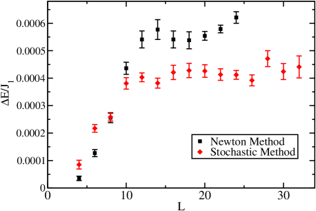
Figure 1: (Color online) The deviation $\Delta E=E_{\rm var}(L)-E_{\rm exact}(L)$ of the variational ground state energy from the exact energy as a function of lattice size. Results obtained with both the Newton method and the stochastic opitimization scheme are shown. The error bars were obtained by carrying out several independent optimization runs for each $L$.

We now discuss our results. In Fig. 1 we compare the ground state energy as calculated with the stochastic and Newton methods. We show the deviations from the correct ground state energies (obtained using unbiased QMC calculations san97 ) as a function of the lattice size $L$ up to $L=32$. Both optimization methods give very small energy deviations for the $4\times 4$ system—about $0.005\%$—but the error grows as the lattice size increases. We have calculated error bars by repeating the optimizations (from scratch) several times. It should be noted, however, that the fluctuations in this kind of nonlinear problem do not necessary have expectation value zero. Hence error bars calculated in the standard way in general only reflect partially the actual errors.

For $L>10$ the stochastic method delivers significantly lower energies, indicating that the Newton method has difficulties in locating the optimum exactly. We believe that this problem is due to the statistical errors of the second derivatives (which are much larger than those of the first derivatives). Convergence issues related to statistical fluctuations of the Hessian are well known in variational calculations for electronic systems.umrigar Any systematic shifts in the Newton method would of course be reduced by increasing the length of the simulation segments used to calculate the energy and its derivatives in each iteration. Simulations sufficiently long to reach the same level of optimization as with the stochastic method do not appear to be practically feasible, however. In the stochastic scheme all statistical errors should decrease to zero as the cooling rate is reduced. We cannot, of course, guarantee that the results shown in Fig. 1 are completely optimal, but we have carried out the simulations at different cooling rates in order to check the convergence. Based on these tests we do believe that the results are converged to their optimum values to within the error bars shown.

For the larger lattices, the energy deviation in Fig. 1 is only $\Delta E/J\approx 0.0004$, or $\approx 0.06\%$, and is size independent within statistical errors for $L>10$. This should then be the accuracy in the thermodynamic limit. In Ref. lia88, only a few of the short-length amplitudes were optimized and a functional form—power-law or exponential—was used for the long-range behavior. The best power-law wave functions had energy deviations of $\Delta E/J\approx 0.0008$; twice as large as we have obtained here with the fully optimized amplitudes.

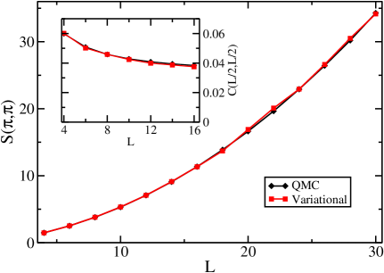
Figure 2: (Color online) The staggered structure factor $S(\pi,\pi)$ versus lattice size, compared with unbiased QMC results. The inset shows the long-distance spin-spin correlation. Statistical errors are smaller than the symbols.

Having concluded that the stochastic method is the preferred optimization technique, we discuss only results for other quantities obtained this way. Fig. 2 shows the size dependence of the staggered structure factor,

$$S(\pi,\pi)=\sum_{x,y}(-1)^{x+y}C(x,y),$$ (18)

where $C(x,y)$ is the correlation function, defined by

$$C(x_{i}-x_{j},y_{i}-y_{j})=\langle{\bf S}_{i}\cdot{\bf S}_{j}\rangle.$$ (19)

The inset shows the correlation function at the longest distance; $(x,y)=(L/2,L/2)$,. We again compare with results from unbiased QMC calculations.san97 The structure factor of the variational ground state agrees very well with the exact result for these lattice sizes—the deviations are typically less than $0.5\%$. The long-distance correlations show deviations that increase slightly with $L$, going to $\approx 2\%$ below the true values for $L\geq 10$ [which then should also be the asymptotic $L\to\infty$ error of $S(\pi,\pi)$]. The sublattice magnetization is the square-root of the long-distance correlation function; it is thus only $1\%$ smaller than the exact value.

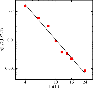
Figure 3: Log-log plot of the amplitude $h(L/2,L/2-1)$ versus the system size. Statistical errors are of the order of the size of the circles. The line shows the power-law $h\sim L^{-3}$.

Liang et al. did not conclusively settle the question of the asymptotic behavior of the amplitudes $h(x,y)$ for bonds of long length $r=(x^{2}+y^{2})^{1/2}$.lia88 The best variational energy was obtained with an algebraic decay; $h\sim r^{-4}$. However, the energy is not very sensitive to the long-distance behavior and the values obtained for $r^{-3}$ and $r^{-2}$ were not substantially different at the level of statistical accuracy achieved. Even with an exponential decay of the bond-length distribution the energy was not appreciably higher, but then no long-range order is possible and hence this form can be excluded. In a recent unbiased projector QMC calculation, the probability distribution $P(x,y)$ of the bonds was calculated.san05 The form $P(r)\sim r^{-3}$ was found (with no discernible angular dependence). Without a hard-core constraint for the VB dimers, the probabilities would clearly be proportional to the amplitudes; $P(x,y)\propto h(x,y)$, and even with the hard-core constraint one would expect the two to be strongly related to each other. In fact, as was pointed out in Ref. san05, , a wave function with $h(r)\sim r^{-p}$ does result in $P(r)\sim r^{-p}$. Our variational calculation confirms that indeed the fully optimized $h(r)\sim r^{-3}$, as demonstrated in Fig. 3 using the longest bonds, $(x,y)=(L/2,L/2-1)$, on the periodic lattices.

Havilio and Auerbach carried out a VB mean-filed calculation which gave an exponent $p\approx 2.7$.havilio2 The statistical accuracy in Fig. 3 is perhaps not sufficient to definitely conclude that $p=3$ exactly, or to exclude $p=2.7$, from this data alone. However, the QMC study of the probability distribution $P(R)$ supports $p=3$ to significantly higher precision.san05 Moreover, Beach has recently developed a different mean-field theory which predicts $p=d+1$ for a $d$-dimensional system. beachmeanfield There is thus reason to believe that $r^{-3}$ indeed is the correct form for $d=2$.

For the $4\times 4$ lattice we can compare the variational wave function with the exact ground state obtained by exact diagonalization. This comparison is most easily done by transforming the VB state to the $S^{z}$ basis. Taking into account the lattice symmetries, there are $822$ $m_{z}=0$ states with momentum $k=0$, and the matrix can easily be diagonalized. We generate the $8!$ VB states $|V_{k}\rangle$ using a permutation scheme and convert each of them into $2^{8}$ $S^{z}$-basis states with weights $\pm\prod h(x,y)$, and use these to calculate the overlap with the exact ground state. With the amplitudes normalized by $h(1,0)=1$, there is only one independent amplitude, $h(2,1)$, to vary for the $4\times 4$ lattice. In Fig. 4 we show the overlap as a function of $h(2,1)$. We also indicate the value of $h(2,1)$ obtained in the variational QMC calculation—it matches almost perfectly that of the maximum overlap. The best overlap is indeed very high; $\approx 0.9998$. It would be interesting to see how the overlap depends on the system size. For a $6\times 6$ lattice, the ground state can also be calculated, using the Lanczos method, but the space of valence bond states is too large to calculate the overlap exactly (although it could in principle be done by stochastic sampling).

  

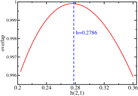
Figure 4: (Color online) Overlap between the exact $4\times 4$ wave function and the VB wave function versus the single independent amplitude $h(2,1)$. The value of $h(2,1)$ obtained in the variational calculation is indicated.

V Frustrated systems

We have also studied the Heisenberg hamiltonian including a frustrating interaction;j1j2

$$H=J_{1}\sum_{\langle i,j\rangle}{\bf S}_{i}\cdot{\bf S}_{j}+J_{2}\sum_{\langle\langle i,j\rangle\rangle}{\bf S}_{i}\cdot{\bf S}_{j},$$ (20)

where $\langle i,j\rangle$ and $\langle\langle i,j\rangle\rangle$ denotes nearest and next-nearest neighbors, respectively, and $J_{1},J_{2}>0$. Also in this case there exists, in principle, a positive-definite expansion of the ground state in the valence bond basis. This can be easily seen because a negative coefficient $f_{k}$ in Eq. (3) can be made positive simply by reversing the order of the indices in one singlet in that particular state. However, no practically useful convention for fixing the order is known. We here use the same partition of the lattice into A and B sublattice sites as in the non-frustrated case and the same sign convention (4) for the singlets. We only consider the $4\times 4$ lattice, which, as we will show, already gives some interesting information on the behavior of the simple amplitude-product wave function as the frustration ratio $J_{2}/J_{1}$ is increased.

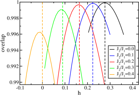
Figure 5: (Color online) Overlap beween the exact $4\times 4$ ground state and the VB wave function for different values of the frustration $J_{2}/J_{1}$. The best amplitudes obtained in variational Monte Carlo calculations are indicated with the dashed lines.

In the exact calculation we can study both positive and negative values of $h(2,1)$, but for now we restrict the variational calculation to $h(2,1)>0$, in order to avoid the Monte Carlo sign problem caused by negative amplitudes.signnote It should be noted, however, that the sign problem here is much less severe than in exact QMC schemes,san05 and hence there is some hope of actually being able to consider mixed signs in variational QMC calculations in the VB basis.signnote

In Fig. 5 we plot the dependence on $h(2,1)$ of the overlap between the VB wave function and the exact ground state for several values of $J_{2}/J_{1}$. The $h(2,1)$ corresponding to maximum overlap decreases as the frustration increases. For $J_{2}/J_{1}=0.4$ the best overlap occurs for $h(2,1)<0$. The optimum overlap decreases significantly with $h(2,1)$ for $J_{2}/J_{1}\gtrsim 0.3$, indicating the increasing effects of bond correlations not taken into account in the product-form of the expansion coefficients. This deterioration of the wave function may be related to the phase transition taking place in this model at $J_{2}/J_{1}\approx 0.4$.j1j2 Note, however, that even at $J_{2}/J_{1}=0.4$ the overlap remains as high as $\approx 0.996$.

There is a point close to $J_{2}/J_{1}=0.4$ where $h(2,1)$ vanishes and thus the best wave function for the $4\times 4$ lattice contains only bonds of length $1$. Beyond this coupling the optimum wave function requires a negative $h(2,1)$. It has also been noted previously that wave functions including only the shortest bonds give the best description of the ground state in a narrow region of high frustration in a model containing also a third-nearest neighbor interaction $J_{3}$.mambrini

We also show in Fig. 5 the values of $h(2,1)$ obtained in the variational calculations. Interestingly, these values coincides well with the maximum overlaps only when the frustration is weak, showing that the best variational state in a given class is not always the best in terms of the wave function.

VI Summary and conclusions

In conclusion, we have shown that a variational valence bond wave function, parametrized in terms of bond amplitude products, gives a very good description over-all of the 2D Heisenberg model. Although this has been known qualitatively for a long time,lia88 our study shows that the agreement is quantitatively even better than what was anticipated in previous studies. The deviation of the ground state energy from the exact value is $\approx 0.06\%$ for large lattices; almost $50\%$ better than in previous calculations where a functional form was assumed for the amplitudes.lia88 The sublattice magnetization is correct to within $\approx 1\%$ (smaller than the true value). We have also shown that the amplitudes for bonds of length $r$ decay as $r^{-3}$ for large $r$, which is the same form as for the probability distribution calculated previously.san05 It is also in agreement with a recently developed mean-field theory.beachmeanfield

By exactly diagonalizing the hamiltonian on a $4\times 4$ lattice, we have also studied the frustrated J₁–J₂ model. Not surprisingly, we found that the quality of the amplitude-product wave function deteriorates when the frustration $J_{2}/J_{1}$ is increased. However, even at $J_{2}/J_{1}=0.4$, i.e., close to the phase transition taking place in this model,j1j2 the overlap is above $0.996$. It would clearly be interesting to see how well the amplitude-product state works for the frustrated model on larger lattices. In this regard we note that Capriotti et al. capriotti recently carried out a variational study of an RVB function written in terms of fermion operators and87 and found that it gave the best description of the ground state of the J₁–J₂ model at large frustration; $J_{2}/J_{1}\approx 0.5$. However, the overlap is significantly smaller than what we have found here for the $4\times 4$ system at the same level of frustration.

Although the fermionic and87 and bosonic descriptions of the VB states are formally equivalent, the fermionic wave function, as it is normally written, does not span the full space possible with the bosonic product state. As a consequence, the bosonic description we have used here can in practice deliver much better variational wave functions for non-frustrated systems.poilblanc The fermionic description apparently works better for frustrated than non-frustrated systems.capriotti However, if the sign is also optimized for each amplitude in the bosonic product state (which is not easy for large highly frustrated systems, however, because of Monte Carlo sign problems signnote ) it is clear that these wave functions should be better than the fermionic RVB state considered so far.capriotti Therefore, the VB wave function we have studied here should, at least in principle, give an even better description of the ground state of the frustrated model than the fermionic RVB state optimized in Ref. capriotti, . Our results for the $4\times 4$ lattice, along with the results of Ref. capriotti, , suggest that the QMC sign problem signnote should be small up to $J_{2}/J_{1}\approx 0.4$. It may thus even be possible to gain insights into the quantum phase transition and the controversial statej1j2 for $J_{2}/J_{1}>0.4$ with this type of variational wave function.

Another interesting question is how bond correlations, which are not included in the wave function considered here, develop as the phase transition at $J_{2}/J_{1}\approx 0.4$ is approached. We are currently exploring the inclusion of bond-pair correlations to further improve the variational wave function for the Heisenberg model as well as more complicated spin models.

The stochastic energy minimization scheme that we have introduced here, which requires only the signs of the first energy derivatives, may also find applications in variational QMC simulations of electronic systems. Recently proposed efficient optimization schemes umrigar ; sorella need the second energy derivatives, and so our scheme requiring only first derivatives has the potential of significant time savings when the number of variational parameters is large. Very recently, other powerful schemes also requiring only the first energy derivatives have been developed and have been shown to be applicable to wave functions with a large number of parameters.umrigar2 We have not yet compared the efficiencies of these different optimization approaches with the stochastic scheme presented here.

- (1) G. Rumer, Göttingen Nachr. Tech. 1932, 377 (1932).
- (2) L. Pauling, J. Chem. Phys. 1, 280 (1933).
- (3) L. Hulthén, Arkiv Mat. Astron. Fysik 26A, No. 11 (1938).
- (4) P. Fazekas and P. W. Anderson, Philos. Mag. 30, 23 (1974).
- (5) P. W. Anderson, Science 235, 1196 (1987); P. W. Anderson, G. Baskaran, Z. Zou, and T. Hsu, Phys. Rev. Lett. 58, 2790 (1987).
- (6) S. Liang, B. Doucot, and P. W. Anderson, Phys. Rev. Lett. 61, 365 (1988).
- (7) C. Gros, Phys. Rev. B 38, 931 (1988).
- (8) D. Poilblanc, Phys. Rev. B 39, 140 (1989).
- (9) N. E. Bonesteel, and J. W. Wilkins, Phys. Rev. Lett. 66, 1232 (1991).
- (10) G. Fano, F. Ortolani, and L. Ziosi, Phys. Rev. B 54, 17557 (1996).
- (11) M. Havilio and A. Auerbach, Phys. Rev. Lett. 83, 4848 (1999).
- (12) M. Havilio and A. Auerbach, Phys. Rev. B 62, 324 (2000).
- (13) L. Capriotti, F. Becca, A. Parola, and S. Sorella, Phys. Rev. Lett. 87, 097201 (2001).
- (14) S. A. Kivelson, D. S. Rokhsar, and J. P. Sethna, Phys. Rev. B 35, 8865 (1987).
- (15) S. Chakravarty, B. I. Halperin, and D. R. Nelson, Phys. Rev. Lett. 60, 1057 (1988); Phys. Rev. B 39, 2344 (1989).
- (16) E. Manousakis, Rev. Mod. Phys. 63, 1 (1991).
- (17) P. L. Iske and W. J. Caspers, Physica A 142, 360 (1987).
- (18) M. Kohmoto, Phys. Rev. B 37, 3812 (1988).
- (19) S. Tang and H. Q. Lin, Phys. Rev. B 38, 6863 (1988).
- (20) B. Sutherland, Phys. Rev. B 37, 3786 (1988).
- (21) S. Liang, Phys. Rev. B 42, 6555 (1990).
- (22) G. Santoro, S. Sorella, L. Guidoni, A. Parola, and E. Tosatti, Phys. Rev. Lett. 83, 3065 (1999).
- (23) A. W. Sandvik. Phys. Rev. Lett 95, 207203 (2005).
- (24) K. S. D. Beach and A. W. Sandvik, Nucl. Phys. B 750, 142 (2005).
- (25) K. S. D. Beach and A. W. Sandvik (manuscript in preparation).
- (26) A. W. Sandvik, cond-mat/0611343.
- (27) K. S. D. Beach and A. W. Sandvik, cond-mat/0612126.
- (28) K. S. D. Beach (unpublished).
- (29) A. W. Sandvik. Phys. Rev. B 56, 11678 (1997).
- (30) T. Barnes and E. S. Swanson, Phys. Rev. B 37, 9405 (1988); J. Carlson, ibid. 40, 846 (1989); M. Gross, E. Sánchez-Velasco, and E. D. Siggia, ibid. 39, 2484 (1989); 40, 11328 (1989); N. Trivedi and D. M. Ceperley, ibid. 40, 2737 (1990); 41, 4552 (1990). K. J. Runge, ibid. 45, 7229 (1992); 45, 12292 (1992). R. A. Sauerwein and M. J. de Oliveira, ibid. 49, 5983 (1994); U.-J. Wiese and H.-P. Ying, Z. Phys. B 93, 147 (1994); B. B. Beard and U.-J. Wiese, Phys. Rev. Lett. 77, 5130 (1996).
- (31) The “Manhattan distance” was used, but very similar results are obtained with .
- (32) W. Press, B. Flannery, S. Teukolsky, W. Vetterling, Numerical Recipes in C++ (Cambridge University Press, 2002).
- (33) C. J. Umrigar and C. Filippi, Phys. Rev. Lett. 94, 150201 (2005).
- (34) C. Peterson and E. Hartman, Neural Networks 2, 475 (1989).
- (35) T. K. Leen and J. E. Moody, Phys. Rev. E 56, 1262 (1997).
- (36) H. Robbins and S. Monro, Ann. Math. Stat. 22, 400 (1951).
- (37) J. C. Spall, in Wiley Encyclopedia of Electrical and Electronics Engineering, Vol. 20, Edited by J. G. Webster (Wiley, 1999).
- (38) A. Harju, B. Barbiellini, S. Siljamäki, R. M. Nieminen, and G. Ortiz, Phys. Rev. Lett. 79, 1173 (1997).
- (39) E. Dagotto and A. Moreo, Phys. Rev. Lett. 63, 2148 (1989); H. J. Schulz, T. Ziman, and D. Poilblanc, J. Phys. I 6, 675 (1996); M. E. Zhitomirsky and K. Ueda, Phys. Rev. B 54, 9007 (1996); O. P. Sushkov, J. Oitmaa, and Z. Weihong, ibid., 63, 104420 (2001); L. Capriotti, F. Becca, A. Parola, and S. Sorella, ibid., 67, 212402 (2003).
- (40) In the fermionic representation of the VB states and87 there is no sign problem in variational calculations poilblanc ; capriotti because the sampling is done using orthogonal basis states. For the VB states we use here, the non-orthogonality leads to sign problems when frustrated interactions are present.
- (41) M. Mambrini, A. Läuchli, D. Poilblanc, and F. Mila, Phys. Rev. B 74, 144422 (2006).
- (42) S. Sorella, Phys. Rev. B 71, 241103(R) (2005).
- (43) C. J. Umrigar, J. Toulouse, C. Filippi, S. Sorella, and R. G. Henning, cond-mat/0611094.