The stochastic dynamics of micron and nanoscale elastic cantilevers in fluid: fluctuations from dissipation

Abstract

The stochastic dynamics of micron and nanoscale cantilevers immersed in a viscous fluid are quantified. Analytical results are presented for long slender cantilevers driven by Brownian noise. The spectral density of the noise force is not assumed to be white and the frequency dependence is determined from the fluctuation-dissipation theorem. The analytical results are shown to be useful for the micron scale cantilevers that are commonly used in atomic force microscopy. A general thermodynamic approach is developed that is valid for cantilevers of arbitrary geometry as well as for arrays of multiple cantilevers whose stochastic motion is coupled through the fluid. It is shown that the fluctuation-dissipation theorem permits the calculation of stochastic quantities via straightforward deterministic methods. The thermodynamic approach is used with deterministic finite element numerical simulations to quantify the autocorrelation and noise spectrum of cantilever fluctuations for a single micron scale cantilever and the cross-correlations and noise spectra of fluctuations for an array of two experimentally motivated nanoscale cantilevers as a function of cantilever separation. The results are used to quantify the noise reduction possible using correlated measurements with two closely spaced nanoscale cantilevers.

I Introduction

The dynamics of micron and nanoscale cantilevers are important to a wide variety of technologies. For example, the invention of the atomic force microscope (AFM) Binnig et al. (1986), which relies upon the dynamics of a cantilever a few hundred microns in length, has revolutionized surface science paving the way for direct measurements of intermolecular forces and topographical mappings with atomic precision for a broad array of materials including semiconductors, polymers, carbon nanotubes, and biological cells Martin et al. (1987); Albrecht et al. (1991); Radmacher et al. (1992); Zhong et al. (1993); Hansma et al. (1994); Garcia and Perez (2002) (see Giessibl (2003); Jalili and Laxminarayana (2004) for current reviews). In conventional dynamic atomic force microscopy the cantilever is used to measure the force interactions between the cantilever tip and sample. Cantilevers smaller than conventional AFM have also been used to unfold single protein molecules with improved force and time resolution Viani et al. (1999). It has also been proposed to exploit the inherent thermal motion of small cantilevers to make dynamic measurements of single molecules arl ; Paul and Cross (2004). A passive undriven cantilever placed in a viscous fluid will exhibit stochastic oscillations caused by the thermal bombardment of fluid molecules by Brownian motion. In fact, measuring the thermal spectra of the cantilever is a commonly used AFM calibration technique Albrecht and Quate (1987); Sader et al. (1999).

In all of these applications the ultimate force sensitivity of a particular measurement is limited by the inherent thermal noise of the experimental system. There are at least two ways to improve upon this limitation: (i) make the cantilevers smaller Walters et al. (1996); Viani et al. (1999), (ii) use correlated measurements of multiple cantilevers Roukes (2000); Paul and Cross (2004).

Uniformly decreasing the dimensions of a cantilever results in the favorable combination of decreasing the cantilever’s equivalent spring constant while increasing its resonant frequency yielding improved force sensitivity and time resolution. By measuring the cross-correlations between two cantilevers in fluid the independent fluctuations of the two do not contribute, leaving only the smaller correlated fluctuations due to coupling through the fluid. This type of approach has been used to measure femtonewton forces on millisecond time scales between two micron scale beads placed in separate optical traps (an improvement of a hundredfold from prior measurements) Meiners and Quake (1999). The ability to significantly increase the force resolution by making correlated measurements has yet to be exploited for micron and nanoscale cantilevers. The magnitude of the fluid coupled noise will depend upon the spacing and exact geometries of the cantilevers. Combining (i) and (ii) and measuring the correlations of multiple nanoscale cantilevers offer the potential for experimental measurements with unprecedented force and time resolution Roukes (2000); Arlett et al. (to appear 2005); Paul and Cross (2004).

As experimental measurement continues to push toward the stochastic limit it is important that we build a physical understanding of the stochastic dynamics of micron and nanoscale cantilevers for the precise conditions of experiment including complex cantilever geometries Albrecht and Quate (1987); Arlett et al. (to appear 2005), the effects of nearby walls Green and Sader (2005); Clarke et al. (2005, 2006); Ma et al. (2000), and the fluid-coupled dynamics of multiple cantilevers in an array configuration Paul and Cross (2004).

Although micron and nanoscale cantilevers exhibit stochastic motion due to the thermal motion of matter the elastic structures are still large compared to individual fluid molecules and the equations of continuum mechanics remain valid. In what follows we are concerned with situations where the Knudsen number (the ratio of the mean free path of the fluid particles to the width of a cantilever) remains sufficiently small so that this statement remains true. This means that the fluid is described by the usual Navier-Stokes equations with no-slip and stress continuity boundary conditions at the solid surfaces.

The Navier-Stokes equations governing the motion of an incompressible fluid, and written in nondimensional form, are

$$R_{\omega}~{}\frac{\partial\vec{u}}{\partial t}+R_{u}~{}\vec{u}{\scriptscriptstyle\stackrel{{\scriptstyle\bullet}}{{{}}}}\vec{\nabla}\vec{u} = -\vec{\nabla}p+\nabla^{2}\vec{u},$$ (1)

$$\vec{\nabla}{\scriptscriptstyle\stackrel{{\scriptstyle\bullet}}{{{}}}}\vec{u} = 0,$$ (2)

where $\vec{u}$ is the fluid velocity, $p$ is the pressure, and $t$ is time. There are two inertial terms on the left hand side of Eq. (1) multiplied by the nondimensional parameters $R_{\omega}$ and $R_{u}$. The Strouhal number $R_{\omega}=L^{2}/\nu T$ plays the role of a frequency based Reynolds number expressing the ratio between local inertia forces and viscous forces where $L$ and $T$ are characteristic length and time scales, respectively. The velocity based Reynolds number $R_{u}=UL/\nu$ expresses the ratio between convective inertial forces and viscous forces.

Micron and nanoscale cantilevers are characterized by high oscillation frequencies and small oscillation amplitudes. In this case $R_{u}\ll 1$ so that the nonlinear convective inertial term $\vec{u}{\scriptscriptstyle\stackrel{{\scriptstyle\bullet}}{{{}}}}\vec{\nabla}\vec{u}$ is negligible and the equations become linear. However, the Strouhal number,

$$R_{\omega}=\frac{\omega w^{2}}{4\nu},$$ (3)

(using the half-width $w/2$ as the appropriate length scale) is often not negligible. As a result, the local inertia term must be kept in Eq. (1) making the analysis more difficult. In addition, experimentally motivated cantilevers are often of complex geometry, near surfaces, or in an array configuration with multiple cantilevers in close proximity. These difficulties have led to the development of a thermodynamic approach to calculate the stochastic dynamics of micron and submicron scale cantilevers for the precise conditions of experiment (discussed below) Paul and Cross (2004). In the following it is assumed that $R_{u}$ is negligible, and we leave off the subscript denoting $R_{\omega}$ by $R$.

The fluid equations are coupled with the governing equations of elasticity,

$$\rho_{c}\frac{\partial^{2}\vec{w}}{\partial t^{2}}=\vec{\nabla}{\scriptscriptstyle\stackrel{{\scriptstyle\bullet}}{{{}}}}\mathbf{\sigma},$$ (4)

where $\sigma$ is the stress tensor, $\rho_{c}$ is the cantilever density, and $\vec{w}(x,y,z,t)$ is the cantilever deflection. Equations (1),(2), and (4) represent the governing deterministic continuum equations. If one considers lengths scales on the order of a few atomic lengths these equations would include stochastic terms Landau and Lifshitz (1959a). This represents a difficult fluid-solid interaction problem governing the stochastic cantilever dynamics. A brute force molecular dynamics approach which would resolve the stochastic motion of all of the fluid and solid molecules is computationally prohibitive. However, the system is always near equilibrium permitting a much more accessible thermodynamic based solution strategy.

The paper is organized as follows. A very general thermodynamic approach, valid for complex geometries as well as for arrays of closely spaced cantilevers, is discussed in Section II. Analytical theory based upon the thermodynamic approach, valid for long slender cantilevers, is discussed in Section III. In Section IV a micron scale cantilever, similar to an atomic force microscope, is explored and in Section V the stochastic dynamics of an array of experimentally motivated nanoscale cantilevers are quantified using the thermodynamic approach with deterministic finite element numerical simulations to generate results for the precise conditions of experiment. A general discussion of the approach can be found in Ref. Paul and Cross (2004).

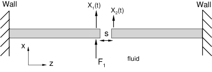
Figure 1: Schematic illustrating an array of two opposing cantilever beams separated by a distance $s$. In the thermodynamic approach of Section II a step force $F_{1}$ is removed from the cantilever on the left and the deterministic cantilever deflections $X_{1}(t)$ and $X_{2}(t)$ are calculated.

II Thermodynamic approach

The thermodynamic approach discussed here is based upon the fluctuation-dissipation theorem which states that for equilibrium systems the manner in which the system returns from a linear macroscopic perturbation is related to time correlations of equilibrium microscopic fluctuations Callen and Welton (1951); Callen and Greene (1952); Chandler (1987). Underlying this statement is the fact that equilibrium fluctuations and the dissipation of the system responding to a macroscopic perturbation are governed by the same physics. For the case of miniature elastic objects in a fluid the dissipation is dominated by the fluid viscosity and the fluctuations by the motion due to the bombardment by the fluid molecules. In what follows, we assume that all of the dissipation comes from the fluid and that elastic dissipation in the cantilever is negligible. This assumption, however, is not required and other sources of dissipation could be included if desired. The essence of our approach is to calculate the dissipation deterministically and to use the fluctuation-dissipation theorem to determine the cantilever’s stochastic dynamics. The approach is exact and the only assumptions that have been made are classical dynamics and linear perturbations from equilibrium. The deterministic calculation of the dissipation can come from analytical theory, simplified models, or from detailed numerical simulations. The major benefit of this approach is that the deterministic calculations are straightforward, not computationally prohibitive, and methods of calculation are sophisticated and readily available.

We will introduce the use of the thermodynamic approach for the case of two opposing cantilevers as shown in Fig. 1. Consider one dynamical variable to be the stochastic displacement of the cantilever on the left $x_{1}(t)$ where $x_{1}(t)$ is a function of the microscopic phase space variables consisting of $3N$ coordinates, $r^{3N}$, and conjugate momenta, $p^{3N}$, of the system and $N$ is the number of particles in the system. The statistical treatment that follows determines the ensemble average of the cantilever deflections $x_{1}(t)$ over all experimental possibilities. For the undisturbed equilibrium system the ensemble average, and correlations, are denoted as $\left<\right>$.

We now take the system to a prescribed macroscopic excursion from equilibrium and observe how the system returns to equilibrium. The macroscopic cantilever deflection as it returns to equilibrium from a prepared initial condition will be denoted as $X_{1}(t)$. For clarity of presentation, lower case variables are reserved for stochastic quantities and upper case variables are for deterministic quantities. The connection between the stochastic and deterministic quantities is particularly straightforward when the excursion from equilibrium is achieved through the application of a step force some time in the distant past that is removed at time $t=0$, i.e. the force given by,

$$f(t)=\left\{\begin{array}[c]{cc}F_{1}&\text{for }t\leq 0\\ 0&\text{for }t>0.\end{array}\right.$$ (5)

The applied force should be conjugate to the variable for which the fluctuations are to be calculated. For the cantilever system under consideration here, to determine the fluctuations of the tip displacements, the force is applied to the tip of the left cantilever. The step force couples with the cantilever deflection $x_{1}(t)$ and the full Hamiltonian of the system $H$ is given by,

$$H=\left\{\begin{array}[c]{cc}H_{0}+\Delta H&\text{for }t\leq 0\\ H_{0}&\text{for }t>0\end{array}\right.$$ (6)

where $\Delta H=-F_{1}x_{1}(t)=-F_{1}x_{1}(0)$ and $H_{0}$ is the unperturbed Hamiltonian. For small perturbations, $F_{1}$, the quantity $\Delta H$ will also be small, and the results are greatly simplified. The nonequilibrium ensemble average $X_{1}(t)$ is given by,

$$X_{1}(t)=\frac{\int dr^{3N}dp^{3N}x_{1}(t)e^{-\beta(H_{0}+\Delta H)}}{\int dr^{3N}dp^{3N}e^{-\beta(H_{0}+\Delta H)}},$$ (7)

where $\beta=(k_{B}T)^{-1}$, $k_{B}$ is Boltzmann’s constant, and $T$ is the absolute temperature. In Eq. (7) the notation $x_{1}(t)$ is used to represent the value of $x_{1}$ evaluated at the phase space coordinates that have evolved from the values $\vec{r}$ and $\vec{p}$ at time $t=0$ Chandler (1987). In the limit of linear perturbations, $\Delta H\ll 1$, this simplifies to,

$$X_{1}(t)=\left<x_{1}\right>+\beta\left<\Delta H\right>\left<x_{1}\right>-\beta\left<x_{1}\Delta H\right>+\mathcal{O}(\Delta H^{2}),$$ (8)

where an equilibrium ensemble average is given by,

$$\left<x_{1}(t)\right>=\frac{\int dr^{3N}dp^{3N}x_{1}(t)e^{-\beta H_{0}}}{\int dr^{3N}dp^{3N}e^{-\beta H_{0}}}.$$ (9)

If we now assume that $x_{1}$ and $X_{1}$ have the equilibrium average $\left<x_{1}\right>$ subtracted and recall that $\Delta H=-F_{1}x_{1}(0)$, we have our desired result,

$$X_{1}(t)=\beta F_{1}\left<x_{1}(t)x_{1}(0)\right>$$ (10)

which can be rearranged to yield,

$$\left<x_{1}(0)x_{1}(t)\right>=k_{B}T\frac{F_{1}}{X_{1}(t)}.$$ (11)

The analysis is similar for the cross correlations of the deflections for two cantilevers in an array,

$$\left<x_{1}(0)x_{2}(t)\right>=\frac{k_{B}T}{F_{1}}X_{2}(t),$$ (12)

where $X_{2}$ is the displacement of tip 2 arising from the step force $F_{1}$ applied to tip 1.

It is interesting to highlight that the cantilever motions are indeed correlated as indicated by Eq. (12). The correlated fluctuations appear contrary to the naive idea that random molecular impacts upon the individual cantilevers should only lead to uncorrelated motion. Additionally, it should be emphasized that the correlated motion of two (or more) cantilevers is no more difficult a calculation than determining the autocorrelation of a single cantilever.

On the left hand side of Eqs. (11) and (12) are stochastic quantities and on the right hand side are deterministic quantities. This permits a significant reduction in effort in the calculations of the auto- and cross-correlations of the cantilever deflections. The macroscopic deflections $X_{1}(t)$ and $X_{2}(t)$ can be found from deterministic theory, model equations, or numerical simulations and the stochastic quantities are found simply through application of Eqs. (11) and (12). The deterministic problem then reduces to the fluid-solid interaction problem given by the removal of a step force on a cantilever. For the step force Eq. (5), for $t<0$, $X_{1}(t)$ has a finite deflection. After the removal of the step force the cantilever returns to its equilibrium position of $X_{1}=0$. The precise manner in which the cantilever returns to equilibrium is dominated by the dissipation in the fluid. An adjacent cantilever will exhibit time dependent deflections given by $X_{2}(t)$. In this case both the initial and final equilibrium deflections are $X_{2}=0$. The motion of the second cantilever is a result of the fluid motion caused by the first cantilever as it returns to equilibrium.

The spectral properties of the auto- and cross-correlations are determined by taking the cosine Fourier transform of Eqs. (11) and (12) with appropriate factors (see Eq. (15)). This yields the noise spectra, $G_{11}(\omega)$ and $G_{12}(\omega)$, given by,

$$G_{11}(\omega) = 4\int^{\infty}_{0}\left<x_{1}(0)x_{1}(t)\right>\cos(\omega t)dt,$$ (13)

$$G_{12}(\omega) = 4\int^{\infty}_{0}\left<x_{1}(0)x_{2}(t)\right>\cos(\omega t)dt,$$ (14)

where $\omega$ is the angular frequency. The noise spectra are precisely the measured quantity in experiment. In the above expression we have defined the spectral density of the random process $y(t)$ to be,

$$G_{y}(\omega)=\lim_{T\rightarrow\infty}\frac{1}{\pi T}\left|\int_{-T/2}^{T/2}[y(t)-\bar{y}]e^{i\omega t}dt\right|^{2},$$ (15)

where $\bar{y}$ is the average of $y(t)$ over time $T$.

In summary, the explicit steps necessary to determine the stochastic dynamics of a cantilever array are:

1. Perform the deterministic calculation. Given some arrangement of cantilevers in a fluid choose one cantilever and apply a step force some time in the distant past. This will eventually result in a finite steady deflection of this cantilever, whereas the other cantilevers will have zero deflection.

2. Remove the step force and calculate the deflections of the cantilevers as a function of time as they return to equilibrium, for two cantilevers this is $X_{1}(t)$ and $X_{2}(t)$ (see for example Fig. 6 for the case of one cantilever). This deterministic calculation can be done analytically or numerically depending upon the complexity of the particular situation.

3. Calculate the stochastic quantities. Using $X_{1}(t)$ and $X_{2}(t)$ calculate the auto- and cross-correlations of the fluctuations from Eqs. (11) and (12). In essence, the cantilever deflections are merely rescaled to produce the stochastic response (this is illustrated by the two ordinate axes in Fig. 6).

4. Use the auto- and cross-correlations to calculate the noise spectra given by Eqs. (13) and (14).

III Analytical theory based on an oscillating infinite cylinder

The equipartition theorem permits the calculation of the mean square mode displacements of micron and nanoscale cantilevers in vacuum Butt and Jaschke (1995). Sader Sader (1998) further developed this approach to include the damping forces of a surrounding viscous fluid and solved the equations of elasticity in the thin beam limit coupled together with the Navier-Stokes equations. He used the approximation that the effect of the fluid on each element of cantilever is the same for an element of a long and slender cantilever moving with the same speed. In the limit of an infinitely long cylinder the flow field around the cantilever can be assumed to be the flow field around an infinite two-dimensional cylinder to a good approximation Sader (1998); Tuck (1969). In addition, because the forces on each element of cantilever due to the fluid depend only on the velocity of that element, and not otherwise on its position in the cantilever, the mode structure of the damped cantilever is unchanged from the undamped limit. We follow this approach here and use the infinite cylinder approximation for the flow field. However we do not assume that the fluid noise is white as was done in Sader (1998) but use the correct spectral density of the Brownian force given by $G_{F}(\omega)$ in Eq. (37). The frequency dependence of the Brownian noise $G_{F}(\omega)$ is determined by the fluid damping $\gamma_{f}(\omega)$ (illustrated in Fig. 2 and discussed further below).

To connect with the previous work we note that the susceptibility $\chi(t)$ connecting the tip displacement to an applied force is given by the cantilever response to a unit impulse of force, which is the derivative of the step force response given by Eq. (11) so that

$$\chi(t)=-\beta\frac{d}{dt}\left<x_{1}(0)x_{1}(t)\right>.$$ (16)

The Fourier transform of $\chi(t)$ is the response to a deterministic sinusoidal force and the imaginary part $\hat{\chi}^{\prime\prime}(\omega)=\text{Im}\left\{\hat{\chi}(\omega)\right\}$, where Im{} indicates the imaginary component is,

$$\hat{\chi}^{\prime\prime}(\omega)=-\beta\int_{0}^{\infty}\frac{d}{dt}\left<x_{1}(0)x_{1}(t)\right>\sin(\omega t)dt,$$ (17)

where we have adopted the Fourier transform convention given by,

$$\hat{x}(\omega) = \int_{-\infty}^{\infty}x(t)e^{i\omega t}dt$$ (18)

$$x(t) = \frac{1}{2\pi}\int_{-\infty}^{\infty}\hat{x}(\omega)e^{-i\omega t}d\omega,$$ (19)

and $i=\sqrt{-1}$. Integrating Eq. (17) by parts and using the definition of the noise spectrum Eq. (13) yields,

$$G_{11}(\omega)=\frac{4k_{B}T}{\omega}\hat{\chi}^{\prime\prime}(\omega).$$ (20)

The susceptibility $\chi(t)$ can be determined by solving for the deterministic cantilever response to a force impulse.

In the following we present results only for the fundamental mode; however higher modes can be included if desired. The equation governing the cantilever motion is then,

$$m_{e}\ddot{X_{i}}+kX_{i}=F_{f}+F_{i},$$ (21)

where the amplitude of the mode displacement is characterized by the tip displacement $X_{i}$, $m_{e}$ is the effective mass of the cantilever in vacuum, $F_{f}$ is the force acting on the cantilever due to the fluid, and $F_{i}=\delta(t)$ is the force impulse ($\delta(t)$ is the Dirac delta). The effective mass of the cantilever $m_{e}$ is chosen to yield the same kinetic energy as in the cantilever mode, and is related to the cantilever mass by,

$$m_{e}=\alpha m_{c},$$ (22)

where $m_{c}$ is the actual cantilever mass and for the fundamental mode of oscillation for a beam $\alpha=0.243$. Taking the Fourier transform of this equation yields,

$$\left(-m_{e}\omega^{2}+k\right)\hat{X_{i}}=\hat{F}_{f}+1.$$ (23)

The force from the fluid can be written in the form,

$$\hat{F}_{f}=m_{cyl,e}\omega^{2}\Gamma(\omega)\hat{x},$$ (24)

where

$$m_{cyl,e}=\alpha m_{cyl}=\alpha\rho_{f}\left(\frac{\pi}{4}w^{2}L\right).$$ (25)

Here $m_{cyl}$ is the effective mass of a fluid cylinder of radius $w/2$ where $\rho_{f}$ is the fluid density, $w$ is the cantilever width, and $L$ is the cantilever length. Again the prefactor $\alpha=0.243$ is to take into account the variation of the fluid force along the cantilever due to the varying velocity given by the mode structure. The fluid loading and damping are captured by the hydrodynamic function $\Gamma(\omega)$ given by,

$$\Gamma(\omega)=1+\frac{4iK_{1}(-i\sqrt{iR})}{\sqrt{iR}K_{0}(-i\sqrt{iR})},$$ (26)

where $K_{1}$ and $K_{0}$ are Bessel functions Rosenhead (1963). In this definition the frequency dependence on the right hand side appears through the frequency dependent Strouhal number $R$.

The cantilever is loaded by the fluid which can be characterized by an effective mass, $m_{f}$, larger than $m_{e}$ that takes into account the fluid mass that is also being moved. The fluid also damps the motion of the cantilever which can be expressed as an effective damping $\gamma_{f}$. Relations for $m_{f}$ and $\gamma_{f}$ can be found by expanding $\Gamma(\omega)$ into its real and imaginary parts in Eq. (23) and rearranging such that,

$$-m_{f}(\omega)\omega^{2}\hat{X_{i}}-i\omega\gamma_{f}(\omega)\hat{X_{i}}+k\hat{X_{i}}=1$$ (27)

to give,

$$m_{f}=\alpha m_{c}\left(1+T_{0}\Gamma^{\prime}\right)$$ (28)

and,

$$\gamma_{f}=\alpha m_{cyl}\omega\Gamma^{\prime\prime},$$ (29)

where $\Gamma^{\prime}$ and $\Gamma^{\prime\prime}$ are the real and imaginary parts of $\Gamma$, respectively. $T_{0}$ is the mass loading parameter, which is the ratio of the mass of a cylinder of fluid with radius $w/2$ to the actual mass of the cantilever, and is given by,

$$T_{0}=\frac{m_{cyl}}{m_{c}}=\frac{\pi}{4}\frac{\rho_{f}w}{\rho_{c}h},$$ (30)

where $\rho_{c}$ is the density of the cantilever and $h$ is the cantilever thickness.

It is evident from Eqs. (28) and (29) that both the fluid loaded mass of the cantilever and the fluidic damping are functions of frequency. The ratio of the mass of the fluid loaded cantilever to the effective mass of the cantilever in vacuum, $m_{e}$, as a function of frequency is given by $m_{f}/m_{e}=1+T_{0}\Gamma^{\prime}(R)$. The factor $T_{0}$ is a constant for any particular choice of cantilever and fluid combination. The frequency dependence of the added mass is then given by $\Gamma^{\prime}(R)$ and is illustrated by the solid line in Fig. 2 and uses the left ordinate axis. The added mass increases rapidly as the frequency is decreased. Over the range of four orders of magnitude in frequency the added mass is seen to change by a factor of approximately 25. The frequency dependence of the fluid damping is given by $\omega\Gamma^{\prime\prime}(\omega)$ and is shown by the dashed line in Fig. 2 using the right ordinate axis. There is a weaker frequency dependence for the fluid damping when compared to the mass loading. The fluid damping decreases as the frequency decreases and over 4 orders of magnitude in frequency the damping changes by a factor of approximately 7.

Figure 2: The frequency dependence of the fluid loaded mass and fluid damping for an oscillating cantilever in a viscous fluid. (solid line) $\Gamma^{\prime}(R)$ illustrates the frequency dependence of the fluid loaded mass. (dashed line) $R\Gamma^{\prime\prime}(R)$ illustrates the frequency dependence of the fluid damping.

Solving for the cantilever response $\hat{X}_{i}(\omega)$ and taking the imaginary part yields,

$$\hat{\chi}^{\prime\prime}=\frac{\omega\gamma_{f}}{(-m_{f}\omega^{2}+k^{2})^{2}-(\omega\gamma_{f})^{2}}.$$ (31)

Using this result in Eq. (20) and rearranging gives the desired result for the spectral density of the stochastic fluctuations in cantilever displacement,

$$G_{11}(\omega)=\frac{4k_{B}T}{k}\frac{1}{\omega_{0}}{\scriptscriptstyle\stackrel{{\scriptstyle\bullet}}{{{}}}}$$

$$\frac{T_{0}\tilde{\omega}\Gamma_{i}(R_{0}\tilde{\omega})}{\left[\left(1-\tilde{\omega}^{2}\left(1+T_{0}\Gamma_{r}(R_{0}\tilde{\omega})\right)\right)^{2}+\left(\tilde{\omega}^{2}T_{0}\Gamma_{i}(R_{0}\tilde{\omega})\right)^{2}\right]},$$

where $\tilde{\omega}=\omega/\omega_{o}$ is a nondimensional reduced frequency, and $R_{0}$ is the Strouhal number evaluated at the resonant frequency in vacuum given by,

$$R_{0}=\frac{\rho_{f}\omega_{0}w^{2}}{4\eta}.$$ (33)

We emphasize that Eq. (III) is not the same as in previous work Sader (1998) which failed to include the frequency dependent of the Brownian force.

To understand the difference from the previous work we now connect Eq. (10) with the calculation in terms of a fluctuating force with spectral density $G_{F}(\omega)$. The fluctuating displacement can be described in terms of the response to this force through the susceptibility

$$G_{11}(\omega)=|\hat{\chi}(\omega)|^{2}G_{F}(\omega).$$ (34)

Inserting Eq. (20) into this expression yields,

$$G_{F}(\omega)=\frac{4k_{B}T}{\omega}\text{Im}\left\{-\frac{1}{\hat{\chi}(\omega)}\right\}.$$ (35)

It is useful at this point to introduce the impedence $Z(t)=F/v$ where $v$ is the velocity of the cantilever tip $\left<\dot{x}_{1}(t)\right>$, it is then straight forward to show,

$$\hat{Z}(\omega)=-\frac{1}{i\omega\hat{\chi}(\omega)}.$$ (36)

Inserting this into Eq. (35) and rearranging yields the desired expression of the fluctuation dissipation theorem,

$$G_{F}(\omega)=4k_{B}T\gamma_{f}(\omega)$$ (37)

where $\gamma_{f}(\omega)=\text{Re}\left\{\hat{Z}(\omega)\right\}$ is the resistance or dissipation and Re{} indicates the real part. For the case of oscillating cantilevers in fluid $\gamma_{f}$ is the effective fluid damping. It is evident from the frequency dependence of the damping that the fluctuating force described by Eq. (37) is not white noise as considered previously Sader (1998) (see Fig. 2 for the variation of $\gamma_{f}$ with frequency).

The spectral density of fluctuations in cantilever displacement $G_{11}(\omega)$ can also be determined by directly solving the governing stochastic equation of motion,

$$m_{e}\ddot{x_{1}}+kx_{1}=F_{f}+F_{B},$$ (38)

where $F_{B}$ is the random force due to Brownian motion. Taking the Fourier transform of this equation yields,

$$\left(-m_{e}\omega^{2}+k\right)\hat{x}=\hat{F}_{f}+\hat{F}_{B}.$$ (39)

Solving for the magnitude of the cantilever response and using Eq. (37) for the spectral density of the Brownian force again yields Eq. (III). Note that integrating this result automatically leads to the equipartition result,

$$\frac{1}{2\pi}\int^{\infty}_{0}G_{11}(\omega)d\omega=\frac{k_{B}T}{k}.$$ (40)

We would like to point out that it is not possible to start with the equipartition result given by Eq. (40) and to then calculate the spectral properties of the fluctuations, one must first start with the fluctuation-dissipation result given by Eq. (37) as done here.

The noise spectrum of the cantilever in fluid may be used to calibrate an AFM. A simple way to do this is to extract the effective spring constant from the the frequency $\omega_{f}$ giving the maximum of the noise intensity. In previous work Sader (1998) the fluctuations of the cantilever have been estimated without the frequency dependence of the numerator in Eq. (III), leading to some inaccuracy in the estimate of the spring constant. Once $\omega_{f}$ is known, the quality factor $Q$ can be estimated from,

$$Q\approx\frac{\omega m_{f}}{\gamma_{f}}=\frac{\frac{1}{T_{0}}+\Gamma_{r}(R)}{\Gamma_{i}(R)},$$ (41)

where Eqs. (28) and (29) have been used for the mass and damping. This expression for $Q$ is only approximate again because the frequency response of the cantilever is not precisely like that of simple harmonic oscillator, since both $m_{f}$ and $\gamma_{f}$ are frequency dependent.

The error incurred by neglecting the frequency dependence in the numerator in Eq. (III) in fitting the spectrum of a Brownian driven cantilever is illustrated in Fig. 3 as a function of $R_{0}$ and $T_{0}$. In Fig. 3 $\omega_{f}^{*}$ is the frequency at the maximum of the noise spectrum when the frequency dependence has not been included (specifically, in Eq. (III) $G_{F}(\omega)$ has been assumed constant) and $\omega_{f}$ is the correct value of the frequency using the fluctuation-dissipation theorem as discussed in Section III. The results indicate that as the Strouhal number increases the error in this assumption becomes smaller. In particular, when the frequency dependence is neglected the approximate theory always underpredicts $\omega_{f}$. This can be understood in light of Fig. 2 where it is clear that the magnitude of the damping decreases as the frequency of oscillation is reduced. When this decrease is not included the predicted value of $\omega_{f}$ will be unnecessarily reduced. Although the fluid induced damping slowly decreases as the oscillation frequency is reduced it is important to note that the fluid loaded mass increases rapidly and it is this interplay which results in the small $Q$ associated with oscillating micron and nanoscale cantilevers.

Figure 3: The error in predicting the frequency at the maximum of the noise spectrum $\omega_{f}^{*}/\omega_{f}$. $\omega_{f}^{*}$ is the predicted frequency at the maximum of the noise spectrum when the frequency dependence of the Brownian force is neglected as done in previous work Sader (1998) and $\omega_{f}$ is the correct value given by the results of Section III. Results are presented as a function of mass loading $T_{0}$ and the Strouhal number $R_{0}$ based upon the cantilever’s resonant frequency in vacuum. The curves are for $R_{0}=128,64,32,16,4,1,0.25,0.0625$ where $R_{0}=0.0625,1,128$ are labelled and the remaining curves are in sequential order.

Figure 4 summarizes the theoretical results and allows for easy determination of the stochastic dynamics of a single cantilever of arbitrary geometry placed in an arbitrary viscous fluid. Given a particular cantilever and fluid combination the procedure is:

1. Determine the cantilever spring constant $k$, resonant frequency in vacuum, $\omega_{0}$, and characteristic length scale. These can be experimental measurements or theoretical calculations. The characteristic length is a measure of the characteristic half-width of the cantilever.

2. Determine $R_{0}$ from Eq. (33) and $T_{0}$ from Eq. (30).

3. Use $R_{0}$ and $T_{0}$ to determine $\omega_{f}/\omega$ from Fig. 4(a) and $Q$ from Fig. 4(b).

Figure 4: Panel (a) the reduced frequency $\tilde{\omega}$ of oscillation for a cantilever undergoing stochastic oscillations in a viscous fluid as a function of mass loading $T_{0}$ and the Strouhal number $R_{0}$ based upon the cantilever’s resonant frequency in vacuum. Panel (b), the quality factor $Q$ as a function of $R_{0}$ and $T_{0}$ as given by Eq. (41). In each panel the largest value of $R_{0}$ is labelled and each successive curve represents $R_{0}/2$, i.e. in panel (a) the last curve is for $R_{0}=0.0625$ and in panel (b) the last curve is for $R_{0}=1/2$.

In the case that the cantilever is driven externally the response can be found in a similar manner. If the cantilever is driven by a force $F_{d}(t)$ the equation of motion becomes,

$$m_{e}\ddot{x}+kx=F_{f}+F_{d}.$$ (42)

If the driving force is $F_{d}=A_{0}\sin(\omega_{d}t)$ where $A_{0}$ is a constant and $\omega_{d}$ is the driving frequency the amplitude of the response is given by,

$$|\hat{x}(\omega_{d})|^{2}=\left(\frac{A_{0}\pi}{k}\right)^{2}{\scriptscriptstyle\stackrel{{\scriptstyle\bullet}}{{{}}}}$$

$$\frac{1}{\left[\left(1-\tilde{\omega}_{d}^{2}\left(1+T_{0}\Gamma_{r}(R_{0}\tilde{\omega}_{d})\right)\right)^{2}+\left(\tilde{\omega}_{d}^{2}T_{0}\Gamma_{i}(R_{0}\tilde{\omega}_{d})\right)^{2}\right]},$$

where $\tilde{\omega}_{d}=\omega_{d}/\omega_{0}$ is the reduced driving frequency. We emphasize that Eqs. (42) and (III) are for externally driven cantilevers and neglect Brownian noise. Eqs. (III) and (III) are similar in that they share a common denominator, whereas the additional frequency dependence in the numerator of Eq. (III) is from the frequency dependence of the Brownian noise.

IV Micron scale beam in fluid

The stochastic dynamics of a micron scale cantilever, similar to what is commonly used in atomic force microscopy, are now quantified (see Fig. 5). The beam is chosen from Chon and Sader Chon et al. (2000) where both theoretical and experimental values are present for comparison. The beam properties are summarized in Table 1,

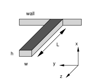
Figure 5: Schematic of a simple cantilevered beam of length $L$, width $w$, and height $h$.

$L$	$w$	$h$	$f_{0}$	$R_{0}$	$T_{0}$
197$\mu$m	29$\mu$m	2$\mu$m	71.56KHz	109.7	4.89

Table 1: The beam geometry: length $L$, width $w$, thickness $h$, resonant frequency in vacuum $f_{0}$, Strouhal number based on the vacuum resonant frequency $R_{0}$ and the mass loading factor $T_{0}$. The beam is silicon with $E=1.74\times 10^{11}$N/m², $\rho_{c}=2320$Kg/m³ and the fluid is water with ($\rho_{f}=997$Kg/m³, $\eta=8.59\times 10^{-4}$Kg/ms). In the deterministic numerical simulations the magnitude of the step force applied is $F_{0}=26$nN.

using classical beam theory Landau and Lifshitz (1959b) the equivalent spring constant $k$ is predicted to be,

$$k=\frac{3EI}{L^{3}},$$ (44)

which yields a value of $k=1.3$N/m and the resonant frequency of the cantilever in vacuum is

$$f_{0}=\frac{C_{1}^{2}}{2\pi L^{2}}\sqrt{\frac{EI}{\mu}},$$ (45)

which yields $f_{0}=71.56$KHz where $C_{1}=1.8751$. Using Eq. (33) the Strouhal number in vacuum is $R_{0}=109.7$ and using Eq. (30) the mass loading factor is $T_{0}=4.89$.

	$Q$	$m_{f}/m_{e}$	$\omega_{f}/\omega_{0}$	$\gamma_{f}$ (kg/s)	$R_{f}$
(1)	3.24	8.16	0.34	$5.07\times 10^{-7}$	37.3
(2)	2.93	8.05	0.35	$6.91\times 10^{-7}$	38.7

Table 2: The stochastic dynamics of a single micron scale cantilever in fluid. (1) Results based on the analytical predictions of Section III. The quality factor $Q$ is calculated from the approximation given by Eq. (41). (2) Results from finite element numerical simulations using the thermodynamic approach of Section II. The numerical results are fit to the simple harmonic oscillator response given by Eq. (47) to determine the listed diagnostics.

We now use the thermodynamic approach to calculate the stochastic dynamics of the cantilever. As previously stated this can be accomplished in a straightforward manner by determining the deterministic response of the cantilever to the removal of a step force applied to the tip. We do this using finite element numerical simulations of the full three dimensional, time-dependent, fluid-solid interaction problem (algorithm discussed elsewhere Yang and Makhijani (1994); cfd ). The simulation is initiated with the removal of a step force applied to the tip of the cantilever and the deterministic dynamics of the beam $X_{1}(t)$ are shown by the solid line in Fig. 6 using the right ordinate axis.

In order to calculate commonly used diagnostics, such as $\omega_{f}$ and $Q$, the deterministic cantilever deflection $X_{1}(t)$ was fit to the deflections of an underdamped simple harmonic oscillator (valid for $Q>1/2$) given by the equation of motion,

$$m_{f}\ddot{X_{1}}(t)+\gamma_{f}\dot{X_{1}}(t)+kX_{1}(t)=0,$$ (46)

where $X_{1}(0)=F_{1}/k$ and $\dot{X_{1}}(0)=0$. The solution is,

$$X_{1}(t)=\frac{F_{1}}{k}e^{-\omega_{f}t/2Q}\left(\cos(\omega^{\prime}t)+\frac{\omega_{f}}{2Q\omega^{\prime}}\sin(\omega^{\prime}t)\right)$$ (47)

where,

$$\omega^{\prime}=\omega_{f}\sqrt{1-\frac{1}{4Q^{2}}},$$ (48)

and $\omega_{f}=\sqrt{k/m_{f}}$. Using a nonlinear least squares curve fit algorithm mat the numerical results are fit to the model to yield the values of $Q$, $\omega_{f}$, $\gamma_{f}$, and $m_{f}$ shown in Table 2. The curve fit is nearly indistinguishable from the numerical simulation results for $X_{1}(t)$ and is shown by the dashed line in Fig. 6.

Using $X_{1}(t)$ in Eq. (11) yields the autocorrelation of the equilibrium deflections, $\left<x_{1}(0)x_{1}(t)\right>$, which are shown in Fig. 6 using the left ordinate axis. The noise spectrum is given by Eq. (13) and is shown in comparison with predictions of the infinite-beam approximation given by Eq. (III) in Fig. 7. The numerical simulations contain all of the oscillation modes as indicated by the presence of the second mode in the figure. In the infinite beam approximation the different modes behave independently and the calculation could be extended to include higher modes if desired. In Table 2 the analytical results of Section III are compared with results using the full thermodynamic approach and deterministic finite element numerical simulations. In general, from the table and the figures, we see that the differences between the simple model and the full calculations are small for this shape cantilever. The experimentally measured value of the resonant frequency in water is $\omega_{f}/\omega_{0}=0.36$ Chon et al. (2000) which agrees well with both the analytical results and the numerical predictions using the thermodynamic approach. However, Table 2 suggests that the analytical results based upon the oscillating infinite cylinder model under predict the amount of damping $\gamma_{f}$. The noise spectra show differences that are small, but may be significant for quantitative applications such as calibration.

In all of the deterministic finite element numerical simulations performed we were careful to ensure that the bounding no-slip surfaces of the computational domain did not affect the results. Comparisons with numerical simulations performed with larger domains did not significantly alter the results.

Figure 6: The dynamics of a micron scale cantilever immersed in water. (solid line) Deterministic finite element numerical simulations using the thermodynamic approach. (dashed line) A simple harmonic oscillator curve fit to the data. The left ordinate yields the autocorrelations of the fluctuations in cantilever displacement and the right ordinate yields the deterministic cantilever dynamics in response to the removal of a step force.

Figure 7: The noise spectrum $G_{11}(\omega)$ for a micron scale cantilever in water. (solid line) Deterministic finite element numerical simulations using the thermodynamic approach. (dashed line) Approximate analytical theory for the fundamental mode only.

V An array of nanoscale cantilevers

As the cantilever dimensions become smaller the effective cantilever spring constant decreases while the resonant frequency increases. This favorable combination potentially provides access to the biologically important parameter regime characterized by 10’s of piconewtons with microsecond scale time resolution, a range that is difficult to reach using other methods. This has led to the development of nanoscale cantilevers Arlett et al. (to appear 2005); Roukes (2000); Craighead (2000).

In what follows we quantify the stochastic dynamics of two adjacent nanoscale cantilevers immersed in water. A schematic of the nanoscale cantilever under consideration here is shown in Fig. 8 Arlett et al. (to appear 2005); Roukes (2000). This is an experimentally motivated cantilever whose paddle shaped geometry decreases the effective spring constant while localizing the strain for piezoresistive measurement. The configuration of the cantilever array is shown in Fig. 1 with two opposing cantilevers separated by a distance $s$. This configuration was chosen because of its experimental accessibility as well as its potential use in single molecule measurements with the tethering of a target biomolecule between the two cantilevers. In the work presented here we build a baseline understanding of the cantilever dynamics in the absence of target biomolecules. Further consideration of the dynamics caused by a tethered biomolecule is beyond the scope of the present paper. The dimensions of the nanoscale cantilevers investigated here are summarized in Table 3.

As discussed previously, the physical properties describing the dynamics of the cantilever in vacuum are important parameters in determining the stochastic dynamics of the cantilevers. These properties are summarized in Table 4 where the values have been determined from finite element simulations of the elastic cantilever structure in the absence of the surrounding fluid. It is important to emphasize that although these calculations can sometimes be performed analytically, this is not the case for many geometries of interest. However, even for cantilevers with very complex geometries, the vacuum based finite element calculations are straight forward.

$L$	$w$	$h$	$L_{1}$	$b$
3$\mu$m	100nm	30nm	$0.6\mu$m	33nm

Table 3: Geometry of the nanoscale cantilever (see Fig. 8). The nanoscale cantilever is composed of silicon ($E=1.25\times 10^{11}$N/m², $\rho_{c}=2330$kg/m³) and the fluid is water ($\rho_{f}=997$kg/m³, $\eta=8.67\times 10^{-4}$kg/ms). The magnitude of the step force applied to the tip of the cantilever is $F_{0}=0.75$pN.

$k$	$\omega_{0}$	$R_{0}$	$T_{0}$
8.7 mN/m	$37.46\times 10^{6}$ rads/s	0.11	1.12

Table 4: The cantilever spring constant $k$, resonant frequency in vacuum $\omega_{0}$, the Strouhal number $R_{0}$, and the mass loading factor $T_{0}$. $\omega_{0}$ and $k$ were determined from numerical simulations of the nanoscale cantilever in vacuum.

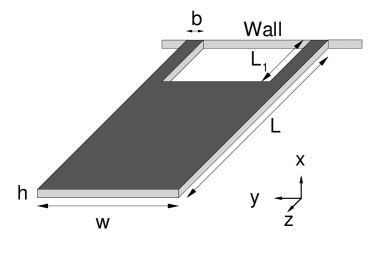
Figure 8: Schematic of an experimentally motivated nanoscale cantilever geometry of length $L$, width $w$, and height $h$.

The stochastic dynamics of the cantilever array are determined using the thermodynamic approach discussed in Section II with deterministic finite element numerical simulations. A series of numerical simulations have been performed to determine the variation in the cantilever dynamics as a function of the separation distance between the two cantilevers in the array. In particular we have explored $s/h=1,2,3,4,5$ where $s$ is the cantilever separation and $h=30$nm is the cantilever thickness. The numerical simulations are initiated by the removal of a step force applied to the tip of one of the cantilevers (in Fig. 1 this is the cantilever on the left) while the other cantilever is initially undeflected and at mechanical equilibrium.

The deterministic dynamics of the nanoscale cantilever for which the step force has been removed, $X_{1}(t)$, is shown by the solid line in Fig. 9 using the right ordinate axis. The deflection $X_{1}$(t) was not significantly affected by the presence of the second cantilever for the separations considered here. As with the micron scale cantilever, we again fit the result for $X_{1}(t)$ from the finite element numerical simulation to the solution of the simple harmonic oscillator equation given by Eq. (46). For the nanoscale cantilever the dynamics are overdamped ($Q<1/2)$ and the deterministic deflection predicted by the simple harmonic oscillator approximation is,

$$X_{1}(t)=\frac{F_{1}}{k}\left(\frac{\lambda_{2}}{\lambda_{2}-\lambda_{1}}e^{\lambda_{1}t}+\frac{\lambda_{1}}{\lambda_{1}-\lambda_{2}}e^{\lambda_{2}t}\right)$$ (49)

where,

$$\lambda_{1,2}=\omega_{f}\left(-\frac{1}{2Q}\pm\sqrt{\frac{1}{4Q^{2}}-1}\right).$$ (50)

The agreement with the curve fit is very good and $\omega_{f}$ and $Q$ are shown in Table 5. Also shown in Table 5 are the theoretical predictions based upon the infinite cylinder approximation. For the analytical calculations of the damping $\gamma_{f}$ from Eq. (29) the fundamental mode of the nanoscale cantilever has been modelled as that of a hinge where all of the bending occurs in the short legs near the base. This is guided by numerical calculations showing the strain localized in the short legs. In this case we find the mass factor is $\alpha=1/3$. (Note that $\alpha$ is not needed to determine the other quantities in Table 5). It is clear from Table 5 that the infinite cylinder approximation is no longer valid. The analytical prediction for the added mass is an order of magnitude too large. This suggests that three-dimensional flow effects become significant for the shape of cantilever under consideration here. For example there would be flow around the tip of the cantilever, as well as the flow through the open region near the base of the cantilever. In addition, the predicted frequency shift is an order of magnitude too small.

	$Q$	$m_{f}/m_{e}$	$\omega_{f}/\omega_{0}$	$\gamma_{f}$ (kg/s)	$R_{f}$
(1)	0.265	106.3	0.032	$2.41\times 10^{-9}$	0.0036
(2)	0.327	18.16	0.236	$1.01\times 10^{-9}$	0.026

Table 5: The stochastic dynamics of a nanoscale cantilever in fluid. (1) Results based on the analytical predictions of Section III. The quality $Q$ is calculated from the approximation given by Eq. (41). (2) Results from finite element numerical simulations using the thermodynamic approach of Section II. The numerical results are fit to the simple harmonic oscillator response given by Eq. (49) to determine the listed diagnostics.

Figure 9: Comparison between the model theory and the full numerical simulation for the autocorrelation of equilibrium fluctuations (right ordinate axis) and the deterministic cantilever deflection relative to the initial deflection of $X_{0}=X_{1}(t=0)$ (left ordinate axis) for a single nanoscale cantilever in fluid: (solid line) results from finite element numerical simulations using the thermodynamic approach; (dashed line) results based upon the approximate analytical theory of Section III.

Inserting $X_{1}(t)$ into Eq. (11) yields the autocorrelation of the equilibrium fluctuations in cantilever displacement, $\left<x_{1}(0)x_{1}(t)\right>$. These are also shown by the solid line in Fig. 9 using the ordinate axis on the left. The noise spectrum, $G_{11}(\omega)$, is found by inserting the autocorrelation in Eq. (13) and the result is shown by the solid line in Fig. 10. Fig. 10 also presents a comparison of the noise spectrum $G_{11}(\omega)$ given from the theoretical predictions of Eq. (III) and the results from the numerical simulations using the thermodynamic approach. The noise spectra are different for small frequencies, in particular the model result has a peak at finite frequency not seen in the full calculation. The inverse cosine transform of the noise spectrum from the infinite-cylinder model yields the deflection of the cantilever as a function of time shown by the dashed line in Fig. 9 using the right ordinate axis. The model prediction for the cantilever deflection exhibits negative values that are not seen in the simulations suggesting that the response of the overdamped cantilever is not precisely that of a simple harmonic oscillator.

Figure 10: The noise spectrum $G_{11}(\omega)$ for a single nanoscale cantilever immersed in water. (solid line) Results from deterministic finite element simulations using the thermodynamic approach described in Section II. (dashed line) Results from approximate analytical theory described in Section III.

We now turn to the deterministic deflection of the second cantilever, $X_{2}(t)$, after removing the force on the first cantilever, evaluated using the full fluid-elasticity simulations. This is shown in Fig. 11 using the right ordinate axis. For close separations $s/h\lesssim 1$ the second cantilever exhibits negative deflections for all time. However, as the cantilever separation increases the second cantilever initially exhibits a positive deflection followed by a negative deflection. The flow field around an oscillating object will have both potential and non-potential components. For an incompressible fluid the potential component is instantaneous whereas the non-potential component diffuses with a diffusion coefficient given by the kinematic viscosity $\nu$. Although the deterministic flow field around simple oscillating objects is well known the fluid coupled motion of multiple elastic objects is not well understood. The fluid dynamics resulting from the motion of two adjacent cantilevers will be discussed in a forthcoming article Clark and Paul .

Using Eq. (12) the stochastic correlations between the two cantilevers can be determined from $X_{2}(t)$. The cross-correlations of the equilibrium displacement fluctuations $\left<x_{1}(0)x_{2}(t)\right>$ are shown in Fig. 11 using the ordinate axis on the left. For small cantilever separations $s/h\lesssim 1$ the cross-correlations are anticorrelated for all time. This is in agreement with experimental measurements of the fluid correlations of two closely spaced micron scale beads in water Meiners and Quake (1999, 2000). However, as the cantilever separation is increased the cross-correlations changes: for short times the cross-correlations are positively correlated whereas for larger times they are anti-correlated.

The noise spectra $G_{12}(\omega)$ are found from $\left<x_{1}(0)x_{2}(t)\right>$ by using Eq. (14). Figure 12 shows the variation in the noise spectra as a function of cantilever separation. The noise spectra contain both positive and negative values and for each cantilever separation there is a frequency at which correlated noise vanishes, $G_{12}(\omega)=0$. This null point could be exploited by a measurement scheme to minimize the correlated noise.

Figure 11: The cross-correlations in equilibrium fluctuations of cantilever deflections for two adjacent nanoscale cantilevers separated by distances $s/h=1,2,3,4,5$ for $h=30$nm found using deterministic finite element numerical simulations with the thermodynamic approach discussed in Section II. The curve for $s/h=1$ is labelled and the others follow in sequential order. The right ordinate axis illustrates the deterministic cantilever deflection as a function of time $X_{2}(t)$ scaled by the deflection of the adjacent cantilever, $X_{0}=X_{1}(t=0$).

Figure 12: The noise spectrum $G_{12}(\omega)$ for two nanoscale cantilevers separated by distance $s/h=1,2,3,4,5$ for $h=30$nm found using deterministic finite element numerical simulations with the thermodynamic approach discussed in Section II. The curve for $s/h=1$ is labelled and the others follow in sequential order.

Figure 13: The force sensitivity and time scales characterizing two adjacent nanoscale cantilevers found using deterministic finite element numerical simulations with the thermodynamic approach discussed in Section II. Panel (a), the maximum magnitude of the force induced by fluid-coupled correlations in cantilever displacement $F_{s}$. The data is empirically fit with an exponential given by $F_{s}=1.12\exp(-0.18s/h)$ (in units of pN). The magnitude of the force felt by a single cantilever due to Brownian noise, $F_{0}=6.0$ pN, is nearly 6 times larger than the correlated noise at close separations ($s/h\lesssim 1$). The right ordinate axis scales $F_{s}$ by $F_{0}$. Panel (b), characteristic time scales, the circles represent the time at which the maximum value of the cross correlation occurs, the squares represent the time at which the fluid induced correlations vanish. The ordinate axis on the right hand side illustrates the time scales when scaled by the period of oscillation of the cantilever in vacuum $t_{0}=(\omega_{0}/2\pi)^{-1}$. The solid lines represent a linear curve fit to the data.

From these results it is possible to characterize the force sensitivity and time resolution of a correlation measurement technique using an array of closely spaced nanoscale cantilevers. An estimate of the force sensitivity can be found using the auto and cross correlation functions as,

$$F_{0} = k||\langle x_{1}(0)x_{1}(t)\rangle||_{max}^{1/2},$$ (51)

$$F_{s} = k||\langle x_{1}(0)x_{2}(t)\rangle||_{max}^{1/2}.$$ (52)

$F_{0}$ represents the approximate magnitude of the stochastic Brownian force acting on a single cantilever and $F_{s}$ the force induced by fluid correlations between two cantilevers. For the case of a single nanoscale cantilever the maximum value occurs at $t=0$ and, using the equipartition theorem this yields a value of $F_{0}=\sqrt{k_{B}Tk}=6.0$pN.

In a cross-correlation measurement between two cantilevers the Brownian noise felt by the two individual cantilevers is uncorrelated and does not contribute. This leaves only the correlations due to the viscous fluidic coupling and $F_{s}$ represents the approximate magnitude of the force due to this hydrodynamic coupling. For example, from Fig. 11 for the case with the closest separation $s/h=1$, the magnitude of the maximum value of the cross-correlation is $\langle x_{1}(0)x_{2}(t)\rangle=1.19\times 10^{-2}$nm² which yields a force sensitivity $F_{s}=0.95$pN. Therefore $F_{s}/F_{0}\approx 1/6$ at $s/h=1$, indicating a 6-fold reduction in thermal noise over a single cantilever measurement.

The variation in $F_{s}$ as a function of cantilever separation is shown in Fig. 13(a). The data is fit with an exponential curve, given by $F_{s}=1.12\exp(-0.18s/h)$ (in units of pN), shown in Fig. 13(a) as the solid line. For very small cantilever separations $s/h\lesssim 1$ the noise reduction possible through the use of a correlated measurement technique is approximately 6-fold. As expected, the correlated noise decreases as the cantilever separation is increased: for a separation of $s/h=5$ there is a 12-fold noise reduction. The ordinate axis on the right hand side of Fig. 13(a) shows $F_{s}/F_{0}$ to show this performance improvement directly.

The characteristic time scales of the fluid correlated motion as a function of cantilever separation are illustrated in Fig. 13(b). In Fig. 13(b) circles represent the time at which the maximum value in the cross correlation occur and squares represent the time at which the fluid induced correlations vanish (i.e., the zero-crossing in Fig. 11). As expected from the finite rate at which momentum diffuses away from an oscillating cantilever, both of these time scales increase with cantilever separation. Using the ordinate axis on the right in Fig. 13(b) the ratio of these time scales to the period of a single oscillation for the cantilever in vacuum $t_{0}=f_{0}^{-1}$ are given.

VI Conclusions

The stochastic dynamics of micron and nanoscale cantilevers can be quantified for the precise conditions of experiment using straightforward deterministic calculations coupled with the fluctuation-dissipation theorem. This can be done for complex cantilever geometries including wall effects, and the stochastic correlated behavior of closely spaced cantilevers for which theoretical predictions currently are not available. Cantilever geometries that are long and thin are well described by approximate analytical theory based upon the oscillation of an infinite cylinder in fluid. We have used the fluctuation-dissipation method to correct the previous results of this theory. For the short and wide nanocantilevers currently being proposed the infinite-cylinder approximation is no longer appropriate. The thermodynamic approach using the fluctuation-dissipation theorem provides an important means of developing a physical understanding of the stochastic dynamics of closely spaced micron and nanoscale objects that will be important as micron and nanotechnology progress and a quantitative design tool for experiment.

This research has been partially supported by DARPA/MTO Simbiosys under grant F49620-02-1-0085 and an ASPIRES grant from Virginia Tech. This work has been carried out in collaboration with the Caltech BioNEMS effort (M. L. Roukes, PI) and we gratefully acknowledge extensive interactions with this team.

References

- Binnig et al. (1986) G. Binnig, C. F. Quate, and C. Gerber, Phys. Rev. Lett. 56, 930 (1986).
- Martin et al. (1987) Y. Martin, C. C. Williams, and H. K. Wickramasinghe, J. Appl. Phys. 61, 4723 (1987).
- Albrecht et al. (1991) T. R. Albrecht, P. Grutter, D. Horne, and D. Rugar, J. Appl. Phys. 69, 668 (1991).
- Radmacher et al. (1992) M. Radmacher, R. Tillman, M. Fritz, and H. Gaub, Science 257, 1900 (1992).
- Zhong et al. (1993) Q. Zhong, D. Inniss, K. Kjoller, and V. Elings, Surf. Sci. 290, L688 (1993).
- Hansma et al. (1994) P. K. Hansma, J. Cleveland, M. Radmacher, D. Walters, P. Hillner, M. Benzanilla, M. Fritz, D. Vie, H. G. Hansma, C. B. Prater, et al., Appl. Phys. Lett. 64, 1738 (1994).
- Garcia and Perez (2002) R. Garcia and R. Perez, Surface Science Reports pp. 197–301 (2002).
- Giessibl (2003) F. J. Giessibl, Reviews of Modern Physics 75, 949 (2003).
- Jalili and Laxminarayana (2004) N. Jalili and K. Laxminarayana, Mechatronics 14, 907 (2004).
- Viani et al. (1999) M. B. Viani, T. E. Schäffer, and A. Chand, J. Appl. Phys. 86, 2258 (1999).
- (11) Arlett et. al., to be published.
- Paul and Cross (2004) M. R. Paul and M. C. Cross, Phys. Rev. Lett. 92, 235501 (2004).
- Albrecht and Quate (1987) T. R. Albrecht and C. F. Quate, J. Appl. Phys 62, 2599 (1987).
- Sader et al. (1999) J. E. Sader, J. W. M. Chon, and P. Mulvaney, Rev. Sci. Instrum. 70, 3967 (1999).
- Walters et al. (1996) D. A. Walters, J. P. Cleveland, N. H. Thomson, P. K. Hansma, M. A. Wendman, G. Gurley, and V. Elings, Rev. Sci. Instrum. 67, 3583 (1996).
- Roukes (2000) M. L. Roukes, Nanoelectromechanical systems, condmat/0008187 (2000).
- Meiners and Quake (1999) J. C. Meiners and S. R. Quake, Phys. Rev. Lett. 82, 2211 (1999).
- Arlett et al. (to appear 2005) J. L. Arlett, M. R. Paul, J. Solomon, M. C. Cross, S. E. Fraser, and M. L. Roukes, in Controlled Nanoscale Motion in Biological and Artificial Systems (Springer-Verlag, to appear 2005), Nobel Symposium 131.
- Green and Sader (2005) C. P. Green and J. E. Sader, Phys. Fluids 17, 073102 (2005).
- Clarke et al. (2005) R. J. Clarke, S. M. Cox, P. M. Williams, and O. E. Jensen, J. Fluid Mech. 545, 397 (2005).
- Clarke et al. (2006) R. J. Clarke, O. E. Jensen, J. Billingham, A. P. Pearson, and P. M. Williams, Phys. Rev. Lett. 96, 050801 (2006).
- Ma et al. (2000) H. Ma, J. Jimenez, and R. Rajagopalan, Langmuir 16, 2254 (2000).
- Landau and Lifshitz (1959a) L. D. Landau and E. M. Lifshitz, Fluid Mechanics (Butterworth-Heinemann, 1959a).
- Callen and Welton (1951) H. B. Callen and T. A. Welton, Phys. Rev. 83, 34 (1951).
- Callen and Greene (1952) H. B. Callen and R. F. Greene, Phys. Rev. 86, 702 (1952).
- Chandler (1987) D. Chandler, Introduction to Modern Statistical Mechanics (Oxford University Press, 1987).
- Butt and Jaschke (1995) H.-J. Butt and M. Jaschke, Nanotech. 6, 1 (1995).
- Sader (1998) J. E. Sader, J. Appl. Phys. 84, 64 (1998).
- Tuck (1969) E. O. Tuck, J. Eng. Math 3, 29 (1969).
- Rosenhead (1963) L. Rosenhead, Laminar Boundary Layers (Oxford University Press, 1963).
- Chon et al. (2000) J. W. M. Chon, P. Mulvaney, and J. E. Sader, J. Appl. Phys. 87, 3978 (2000).
- Landau and Lifshitz (1959b) L. D. Landau and E. M. Lifshitz, Theory of elasticity (Butterworth-Heinemann, 1959b).
- Yang and Makhijani (1994) H. Q. Yang and V. B. Makhijani, AIAA-94-0179 pp. 1–10 (1994).
- (34) CFD Research Corporation, 215 Wynn Dr. Huntsville AL 35805.
- (35) Matlab, The Math Works.
- Craighead (2000) H. Craighead, Science 290, 1532 (2000).
- (37) M. T. Clark and M. R. Paul, unpublished.
- Meiners and Quake (2000) J. C. Meiners and S. R. Quake, Phys. Rev. Lett. 84, 5014 (2000).