Interaction driven real-space condensation

Abstract

We study real-space condensation in a broad class of stochastic mass transport models. We show that the steady state of such models has a pair-factorised form which generalizes the standard factorized steady states. The condensation in this class of models is driven by interactions which give rise to a spatially extended condensate that differs fundamentally from the previously studied examples. We present numerical results as well as a theoretical analysis of the condensation transition and show that the criterion for condensation is related to the binding-unbinding transition of solid-on-solid interfaces.

Real-space condensation has been observed in a variety of physical contexts such as cluster aggregation MKB98 , jamming in traffic and granular flow OEC98 ; CSS00 and granular clustering MWL02 . The characteristic feature of these systems is the stochastic transport of some conserved quantity, to be referred to as mass; the condensation transition is manifested when above some critical mass density a single condensate captures a finite fraction of the mass. The condensate corresponds to a dominant cluster or a single large jam in these examples. Perhaps more surprising realisations of condensation are wealth condensation in macroeconomies BJJKNPZ , where the condensate corresponds to a single individual or enterprise owning a finite fraction of the wealth; condensation in growing or rewiring networks where a single hub captures a finite fraction of the links DM03 and phase separation dynamics in one-dimensional driven systems where condensation corresponds to the emergence of a macroscopic domain of one phaseKLMST02 .

Mass transport may be modelled in terms of interacting many-particle systems governed by stochastic dynamical rules. Generically these systems lack detailed balance and thus have nontrivial nonequilibrium steady states. Although our understanding of such steady states is still at an early stage, a class of models has been determined which exhibit a factorised steady state (FSS) EMZ04 which can be written as a product of factors, one factor for each site of the system. This simple form for the steady state has afforded an opportunity to study condensation analytically and has also been used as an approximation to more complicated nonequilibrium steady states. The conditions under which condensation can occur have been determined, leading to conditions on the stochastic mass transport rules for condensation to result MEZ05 . One key feature of the condensate arising in these models is that it forms at a single site.

In the physical systems of the kind described above, generically the stochastic transport rules depend not only on the departure site but also on the surrounding environment. In general such models do not have FSS and finding their steady states has remained a challenge.

The purpose of this letter is twofold. First, we introduce a broad class of mass transport models where the transport rules depend on the environment of the departure site. These models do not have an FSS, yet we can determine their steady states explicitly. The structure of the steady state generalises the FSS to a pair-factorised steady state (PFSS). Secondly, we find that the nature of the condensate in PFSS is strikingly different from that of the FSS: unlike in the FSS, the condensate is spatially extended. This is due to the short-range correlations inherent in the PFSS, but absent in the FSS.

We consider a class of mass transport models on a periodic chain with sites labelled by $i=1,\ldots,L$. At each site resides a non-negative integer number, $m_{i}$, of particles each of unit mass. We define particle dynamics such that a particle hops from site $i$ to $i{+}1$ with a rate $u(m_{i{-}1},m_{i},m_{i{+}1})$ (provided $m_{i}>0$), so the total mass $\sum_{i}m_{i}=M$ is conserved. These dynamics drive a current of particles through the system.

If the hop rate is only a function, $u(m_{i})$, of mass at the departure site $m_{i}$, the model reduces to the zero-range process EH05 which has a FSS. Explicitly, the probability of a configuration $\{m_{i}\}$ occurring in the steady state is

$$P[\{m_{i}\}]\propto\prod_{i=1}^{L}f(m_{i})\delta\left(\sum_{i}m_{i}-M\right)$$ (1)

where $f(m)=1/\prod_{k=1}^{m}u(k)$ for $m\geq 1$ and $f(0)=1$. Thus there is one factor $f(m_{i})$ for each site $i$ of the system and the delta function ensures that the total mass is $M$.

When the hop rates $u(m_{i{-}1},m_{i},m_{i{+}1})$ depend on all three arguments, we propose the PFSS as a natural generalization of the FSS which takes the following form: the steady state probability of configuration, $\{m_{i}\}$, is

$$P[\{m_{i}\}]=Z_{L,M}^{-1}\prod_{i=1}^{L}g(m_{i},m_{i{+}1})\,\delta(\sum_{i=1}^{L}m_{i}-M)\;.$$ (2)

Thus there is one factor $g(m_{i},m_{i{+}1})$ for each pair of neighbouring sites. The normalisation, $Z_{L,M}$, which plays a role analogous to the canonical partition function in equilibrium statistical mechanics, is given by

$$Z_{L,M}=\sum_{\{m_{i}\}}\prod_{i=1}^{L}g(m_{i},m_{i{+}1})\,\delta(\sum_{i=1}^{L}m_{i}-M)\;.$$ (3)

Note that in the case $g(m_{i},m_{i+1})=f(m_{i})$, for example, the PFSS Eq. (2) reduces to the FSS form (1).

We first establish that the steady state (2) holds for a broad class of mass transport models. We find that if (though not only if) the hop rates out of site $i$ factorize tbp :

$$u(m_{i{-}1},m_{i},m_{i{+}1})=\alpha(m_{i{-}1},m_{i})\beta(m_{i},m_{i{+}1})\;,$$ (4)

then the steady state is of the PFSS form (2) with

$$g(m,n)=\prod_{i=1}^{n}\alpha(m,i)^{-1}\prod_{j=1}^{m}\beta(j,0)^{-1}\;,$$ (5)

for $m,n>0$ where $g(0,0)=1$, provided $\alpha$ and $\beta$ satisfy the constraint

$$\frac{\alpha(m{-}1,n)}{\alpha(m,n)}=\frac{\beta(m,n{-}1)}{\beta(m,n)}\;.$$ (6)

Furthermore given any form of the weight $g(m,n)$ one can determine the functions $\alpha$ and $\beta$ through the following recursions

$$\alpha(l,m)=\frac{g(l,m{-}1)}{g(l,m)}\;,\quad\beta(m,n)=\frac{g(m-1,n)}{g(m,n)}\;.$$ (7)

Thus for every choice of $g(m,n)$ there exists a stochastic mass transport model which will generate the corresponding PFSS.

We now focus on a particular model which has a PFSS with $g(m,n)$ given by

$$g(m,n)=\exp\left[-J|m-n|+\frac{1}{2}U_{0}\left(\delta_{m,0}+\delta_{n,0}\right)\right]\;.$$ (8)

One can check from (7,4) that the corresponding hop rates are

$$u(l,m,n)=\left\{\begin{array}[]{ll}\exp\left[-2J+U_{0}\delta_{m,1}\right]\;,&{\rm for}\quad m\leq l,n\\ \exp\left[2J+U_{0}\delta_{m,1}\right]\;,&{\rm for}\quad m>l,n\\ \exp\left[U_{0}\delta_{m,1}\right]\;.&\quad{\rm otherwise}\end{array}\right.$$ (12)

Physically, the rate is low if the mass at the departure site is less than the neighboring masses and is high if the mass is larger than the neighboring masses. This tends to flatten the density profile and generates the effective surface tension $J$ in (8) implying short-range correlations between the sites. In addition, isolated particles tend to hop relatively quickly leading to a preference in the steady state weights for vacant sites. This is reflected by the on-site attractive potential $-U_{0}\delta_{m_{i},0}$ in (8).

The model defined by the hop rates (12) is guaranteed to have a PFSS with $g(m,n)$ in (8). To investigate whether the model allows for a condensation transition as the parameters $J,U_{0}$ and the conserved mass density $\rho=M/L$ are varied, we have run Monte Carlo simulations, according to the following prescription. The system is prepared in a random, homogeneous initial condition and evolves under random sequential update. During each time step $\delta t$ a site $l$ is selected randomly and if a particle is present it is transferred to the neighbouring site $l{+}1$ with probability $u(m_{l{-}1},m_{l},m_{l{+}1})\,\delta t$. $L$ such time steps constitute a single Monte Carlo step.

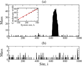
Figure 1: Typical steady state configurations for $L=1000$ and $J=U_{0}=1$ (for which $\rho_{c}=0.51$) in (a) condensed phase, $\rho=3$, and (b) fluid phase $\rho=1/4$. The inset in (a) shows an $L^{1/2}$ dependence (indicated by the solid line) of the condensate width on system size.

We find that two phases emerge in the steady state depending on $\rho$ and $J$ (where we set $U_{0}=1$). As illustrated in Fig.1, at low density the system resides in a fluid phase, in which particles are distributed homogeneously throughout the system. When the density exceeds a critical value $\rho_{c}(J)$, the system is in a condensed phase wherein a condensate containing the excess mass $(\rho-\rho_{c})L$ coexists with a critical background fluid of mass $\rho_{c}L$. In contrast to a usual condensate that occupies a single site, as for example in an FSS, the condensate here extends over many sites. In fact, the condensate extends over typically $O(L^{1/2})$ sites as shown in Fig.1 (a).

To locate the phase boundary in the $\rho$–$J$ plane we computed the single-site probabilities $p(m,L)$ that a site contains exactly mass $m$ in the steady state. In the fluid phase $p(m,L)$ decays exponentially for large $m$ whereas in the condensed phase an additional bump emerges at the large $m$ tail of $p(m,L)$ as illustrated in Fig. 2.

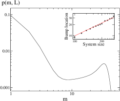
Figure 2: Single-site distribution $p(m,L)$ for a system of $L=1000$ sites with $\rho=3$ and $J=U_{0}=1$. The inset shows the mass at the maximum of the condensate bump as a function of system size $L$, where the crosses are obtained from Monte Carlo simulation and the solid line shows an $L^{1/2}$ dependence.

The phase boundary in Fig. 3 is determined by the value of $J$, for fixed $\rho$, at which a bump in $p(m,L)$ first appears as one increases $J$.

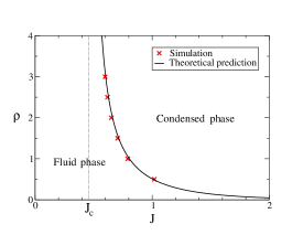
Figure 3: Phase diagram for $U_{0}=1$. The crosses are data points obtained from Monte Carlo simulation. The solid line gives the theoretical prediction (17). For $J<J_{c}$ given by (15) condensation does not occur at any density.

Our theoretical prediction for the phase boundary, presented below, is in excellent agreement with the numerical results.

The condensate bump in $p(m,L)$ also has an interesting scaling behavior with $L$. We plot in the inset of Fig. 2 the mass at the maximum of the bump as a function of $L$ and find that it grows as $L^{1/2}$. This implies that a typical site inside the condensate has mass of order $L^{1/2}$. On the other hand since the condensate carries total excess mass $(\rho-\rho_{c})L$ this implies that there are typically of order $L^{1/2}$ sites inside the condensate i.e. the spatial extent of the condensate is of order $L^{1/2}$.

We now analyze the general conditions under which the steady state (2) may admit condensation. The grand canonical partition function, ${\mathcal{Z}}_{L}(\mu)$ (the Laplace transform of $Z_{L,M}$ with respect to $M$) is given by

$${\mathcal{Z}}_{L}(\mu)=\sum_{\{m_{i}\}}{\rm e}^{-\mu\sum_{i}m_{i}}\prod_{i=1}^{L}g(m_{i},m_{i{+}1})\;,$$ (13)

where the chemical potential $\mu$ is determined from the condition that

$$\rho=\rho(\mu)\equiv-\frac{1}{L}\frac{\partial{\rm ln}\;{\mathcal{Z}}_{L}(\mu)}{\partial\mu}\;,$$ (14)

Clearly $\rho(\mu)$ is a decreasing function of $\mu$ for $\mu\geq 0$ footnote . If, as $\mu\to 0$, the function $\rho(\mu)\to\infty$, then a solution $\mu>0$ of (14) exists for any $\rho>0$. This implies from (13) that the single-site mass distribution decays exponentially for large $m$ signifying a fluid phase and there is no condensation. On the other hand, if, as $\mu\to 0$, the function $\rho(\mu)$ approaches a finite value $\rho_{c}$, then a solution of (14) can only be found for $\rho<\rho_{c}$ implying that the fluid phase exists only for $\rho<\rho_{c}$. When $\rho$ exceeds the critical particle density $\rho_{c}$ there is no solution to (14) implying the onset of condensation wherein the ‘excess’ mass $(\rho-\rho_{c})L$ is carried by the condensate.

Thus to determine if there is condensation one needs to analyze (13) and (14) as $\mu\to 0$. But, for $\mu=0$, (13) is precisely the grand canonical partition function of a solid-on-solid (SOS) interface model CW81 ; vLH81 where the interface height at site $i$ is equivalent to the mass $m_{i}$. Since $m_{i}\geq 0$ the interface heights are strictly non-negative implying that the interface grows on a substrate at $m_{i}=0$. Thus $\rho(0)$ from (14) corresponds to the average interface height $\langle m_{i}\rangle$ in this SOS model. If $\rho(0)=\infty$, i.e. there is no condensation transition, the interface is unbound since its mean height is divergent. On the other hand if there is a condensation transition, in which case $\rho(0)=\rho_{c}$ is finite, the interface is bound with a finite mean height $\rho(0)$. Therefore the criterion for a condensation transition is that the corresponding interface should be bound. Moreover the critical density $\rho_{c}$ is given by the mean height of the bound interface.

We now present an exact calculation of the phase diagram in Fig. 3. The mean height of this SOS interface model can be easily calculated using a standard transfer matrix formalism. The partition function (13) may be written as ${\mathcal{Z}}_{L}(\mu)={\rm Tr}\left[T^{L}(\mu)\right]$ where the elements of the transfer matrix $T$ are $g(m^{\prime},m)$. In the large $L$ limit only the eigenvector $|\phi_{0}\rangle$ of $T$ with the largest eigenvalue $\lambda_{0}$ contributes. The eigenvalue equation reads $\sum_{m=0}^{\infty}g(m^{\prime},m)\langle m|\phi_{\alpha}\rangle=\lambda_{\alpha}\langle m^{\prime}|\phi_{\alpha}\rangle$. The eigenvectors are either extended states $\langle m|\phi_{\alpha}\rangle\sim{\rm e}^{ipm}$ or a bound state $\langle m|\phi_{\alpha}\rangle\sim t^{m}$ where $|t|<1$ CW81 . If the spectrum contains a bound state then the bound state corresponds to the largest eigenvalue. Substituting $\langle m|\phi_{0}\rangle=t^{m}$ into the eigenvalue equation for $m^{\prime}>0$ and $m^{\prime}=0$ separately yields $t={\rm e}^{-J}/(1{-}{\rm e}^{-U_{0}})$. For the bound state to exist $|t|<1$ which implies

$$J>J_{c}=U_{0}-{\rm ln}({\rm e}^{U_{0}}-1)\;.$$ (15)

Therefore, for $J<J_{c}$ the system will not condense at any finite density implying $\rho_{c}=\infty$, whereas for $J>J_{c}$, the system condenses above a finite density $\rho_{c}$. The density $\rho_{c}$ is given by the mean height in the bound state

$$\rho_{c}=\frac{\sum_{m}m|\langle m|\phi_{0}\rangle|^{2}}{\sum_{m}|\langle m|\phi_{0}\rangle|^{2}}\;.$$ (16)

Using the bound state eigenfunction one finds

$$\rho_{c}=\left[{\rm e}^{2(J-J_{c})}-1\right]^{-1}\;.$$ (17)

This prediction is in excellent agreement with the numerical data as illustrated in Fig. 3.

We now discuss the condensation transition in a more general PFSS where

$$g(m,n)=K(|m-n|)\exp\left[\frac{1}{2}\left(U(m)+U(n)\right)\right]\;.$$ (18)

Here $K(|m-n|)$ represents the interaction between nearest neighbor masses and $-U(m)$ is an on-site potential. If $K(x)$ decays sufficiently rapidly for large $x$, as in (8), for condensation to happen one only requires $U(m)$ to be positive and localised near $m=0$. In this case the condensation is interaction-driven and the existence of the condensation transition corresponds to having a bound interface. In such cases quite generically the height and width of the condensate are expected to scale as $L^{1/2}$. This follows from a Brownian excursion argument: the localized on-site potential plays no role at sites occupied by the condensate — in the absence of the potential, the problem can be related to a random walk problem where the random walker takes independent steps with length drawn from a distribution $K(x)$SM06 . The shape of the condensate is determined by a single large loop defined by the excursion of the random walker as shown in Fig. 1. The probability that the walker returns to the origin for the first time after $N$ steps scales as $N^{-3/2}$ for sufficiently rapidly decaying $K(x)$. So, the average number of steps until the first return is $\int_{1}^{L}N^{-3/2}N\;dN\sim L^{1/2}$ (the upper cut-off, $L$, is determined by the maximum number of possible steps). This predicts that the spatial extent of the condensate is ${\mathcal{O}}(L^{1/2})$. Also, because it is Brownian, the typical height of the excursion, and therefore that of the condensate, scales as $L^{1/2}$. Note that the area under the excursion, equivalent to the mass contained in the condensate, is ${\mathcal{O}}(L)$, as it should be.

This interaction-driven condensation is rather different from the type exhibited in an FSS. There the function $K(x)=1$ and a localized on-site attractive potential is no longer capable of driving condensation. Instead one requires a specific unbounded potential of the form $-U(m)\sim\gamma\ln m$ for large $m$ EH05 . Thus in the FSS condensation is potential-driven.

To summarize, the steady state (2) extends the class of exactly solvable steady states in nonequilibrium statistical mechanics. The condensed phase which emerges in a PFSS is fundamentally different from that of an FSS. In a PFSS the condensation is interaction-driven and moreover the condensate extends spatially over ${\mathcal{O}}(L^{1/2})$ sites. The explicit form of the single-site mass distribution $p(m,L)$ in the FSS condensed phase has been determined recently MEZ05 . It remains a challenge to compute $p(m,L)$ for the PFSS condensed phase. It would also be of interest to study PFSS in higher dimensions.

Finally we note that the FSS has provided insight into number of issues of nonequilibrium statistical physics. Although we have focussed here on the issue of condensation, the generalisation to a PFSS should allow one to address other interesting issues such as the role of conservation laws GS03 , disorder K00 , boundary-induced phenomena LMS05 and fluctuation theorems HRS05 .

T. H. thanks the EPSRC for support under programme grant GR/S10377/01.

References

- (1) S. N. Majumdar, S. Krishnamurthy and M. Barma, Phys. Rev. Lett. 81, 3691 (1998)
- (2) O.J. O’Loan, M.R. Evans and M.E. Cates, Phys. Rev. E 58, 1404 (1998).
- (3) D. Chowdhury, L. Santen and A. Schadschneider, Physics Reports 329, 199 (2000)
- (4) D. van der Meer, K. van der Weele and D. Lohse, Phys. Rev. Lett. 88, 174302 (2002)
- (5) Z. Burda etal Phys. Rev. E 65, 026102 (2002)
- (6) S. N. Dorogovstev and J. F. F. Mendes, Evolution of Networks (OUP, Oxford, 2003)
- (7) Y. Kafri, E. Levine, D. Mukamel, G. M. Schütz and J. Török, Phys. Rev. Lett. 89, 035702 (2002)
- (8) M. R. Evans, S. N. Majumdar and R. K. P. Zia, J. Phys. A 37, L275 (2004); ibid 39, 4859 (2006)
- (9) S. N. Majumdar, M. R. Evans and R. K. P. Zia, Phys. Rev. Lett. 94, 180601 (2005); M. R. Evans, S. N. Majumdar and R. K. P. Zia , J. Stat. Phys. 123, 357 (2006)
- (10) M. R. Evans and T. Hanney, J. Phys. A: Math. Gen 38, R195 (2005)
- (11) M. R. Evans, T. Hanney and S. N. Majumdar to be published
- (12) Strictly, if contains a pure exponential factor e.g. , in (13) would exist for ; but this just amounts to a shift in the zero of the chemical potential.
- (13) S. T. Chui and J. D. Weeks, Phys. Rev. B 23, 2438 (1981)
- (14) J. M. J. van Leeuwen and H. J. Hilhorst, Physica A 107, 319 (1981); T. W. Burkhardt, J. Phys. A 14, L63 (1981)
- (15) G. Schehr and S. N. Majumdar, cond-mat/0601073
- (16) S. Grosskinsky and H. Spohn, Bull. Braz. Math. Soc. 34, 1 (2003); M. R. Evans and T. Hanney, J. Phys. A: Math. Gen 36, L441 (2003)
- (17) J. Krug, Braz. J. Phys. 30, 97 (2000); K. Jain and M. Barma, Phys. Rev. Lett. 91, 135701 (2003)
- (18) E. Levine, D. Mukamel and G. M. Schütz, J. Stat. Phys. 120, 759 (2005)
- (19) R. J. Harris, A. Rákos and G. M. Schütz, J. Stat. Mech. P08003 (2005)