Monte Carlo simulation of size-effects on thermal conductivity in a 2-dimensional Ising system

Abstract

A model based on microcanonical Monte Carlo method is used to study the application of the temperature gradient along a two-dimensional (2D) Ising system. We estimate the system size effects on thermal conductivity, $K$, for a nano-scale Ising layer with variable size. It is shown that $K$ scales with size as $\ K=cL^{\alpha}$ where $\alpha$ varies with temperature. Both the Metropolis and Cruetz algorithms have been used to establish the temperature gradient. Further results show that the average demon energy in the presence of an external magnetic field is zero for low temperatures,
PACS numbers: M68.65.-k., 68.65.Ac.
Keywords: Monte Carlo simulation, Ising system, thermal conductivity.

1 Introduction

The Ising system was introduced many decades ago to study simple spin systems. Over the years it has stood the test of time and proved to be useful in many areas of physics, from statistical mechanics to biological systems [1]. As such, it has also been in use to study large scale Monte-Carlo (MC) simulations of complex systems ever since the advent of adequate computing power to tackle such challenges. As is well known, the usual MC algorithm is a useful approximation if the time scales over which thermal diffusion occurs are very short. It is therefore clearly inadequate for problems where the dynamical process is controlled by local variations in temperature, including the calculation of thermal conductivity. To avoid such shortcomings, Creutz [2] developed a micro-canonical algorithm by introducing “demons” to control distribution of energy throughout the system. Such demons may be conceived to act as thermometers. This is particularly helpful in performing non-equilibrium simulations with unequal local temperatures. This development was the basis of thermal conductivity computations in a 2D Ising system presented in [3]. The same method was further developed later by Mak [4] to accommodate external magnetic fields.

In this paper we use the Creutz algorithm together with Fourier law to calculate thermal conductivity within the framework of a 2D Ising system. In doing so, we have also investigated the size effects and shown that thermal conductivity scales as $\ K=cL^{\alpha}$ where $\alpha$ varies with temperature and $L$ is the size of the system. We further show that the average demon energy when an external magnetic field is present is zero at low temperatures. Also, the demon thermometer, as developed by Mak, leads to unacceptable temperature gradients. However, this thermometer works satisfactorily at high temperatures.

2 Ising model and thermal conductivity

Let us first briefly consider the salient features of the Ising system in 2D relevant to our present discussion. This model is characterized by the interaction Hamiltonian $H$ given by

$$H=\frac{J}{2}\sum_{i}\sum_{j\neq i}{S_{i}}{S_{j}}\,-\,h\sum_{i}{S_{i}},$$ (1)

where the spin variables $\ S_{i}$ take values from the set $\{1,-1\}$ with $\frac{1}{2}$ denoting the set of all nearest neighbor pairs and $h$ is proportional to a uniform external magnetic field. The exchange constant $J$ is a measure of the strength of the interaction between nearest neighbor spins. If $J<0$, we expect the state of the lowest total energy to be ferromagnetic, i.e. the spins all point in the same direction. For $J>0$, the state of the lowest energy is expected to be anti ferromagnetic, that is, alternate spins are aligned. Here we concentrate on the ferromagnetic case. A particular configuration of microstates of the lattice is specified by the set of variables $\{S_{1},S_{2},\cdots,S_{n}\}$ for all lattice sites. We work with units in which $1/T=\beta$.

2.1 Thermal conductivity from Monte Carlo simulations

The method we have used is based on the micro-canonical algorithm of Creutz which is complementary to the standard Monte Carlo method. Here, we investigated the transport properties in a non-equilibrium steady state. Let us first note that as temperature is an incoming parameter to the metropolis algorithm, having been fixed before hand, the system changes with a fixed temperature and there would be no possibility to explore the behavior of the system if the temperature changes from one part of the system to the other. However, if we were to study a system with local temperature variations, we would be able to compute such transport coefficients as thermal conductivity. Creutz has shown that the method can also be used for dynamical properties, in a qualitative study of thermal conductivity [2].

To this and other ends, we first divide our 2D system and make it into many sub-layers. We then equilibrate the system (all layers) at temperature $T_{m}$ using Metropolis algorithm and as usual, periodic boundary conditions are used along each direction. After equilibration we select a few layers from each end and fix their temperatures at $T_{h}$ ($h$ for high) and $T_{l}$ ($l$ for low) using Metropolis algorithm. At this point we have to remove periodic boundary condition in the $x$-direction, i.e. along the direction for which a temperature gradient is expected. We apply periodic boundary conditions along the direction for which there is no temperature gradient, that is, the $y$-direction. Also note that $T_{m}=\frac{T_{h}+T_{l}}{2}$ and the symbol $T$ instead of $T_{m}$ has been used in all the figures. After many iterations we can calculate thermal conductivity of the system at $T_{m}$ using the Fourier’s law for heat conduction [5]. The temperature gradient is then deduced from the resulting linear temperature profile, that is, from the Fourier law

$${\bf Q}=-K{\bf\nabla}T({\bf x},t),$$ (2)

where ${\bf Q}$ is the heat current and $K$ is the thermal conductivity of the system.

To study the behavior of a temperature gradient, we use the “demon algorithm” [2]. To understand the mechanism behind this algorithm suppose we add an extra degree of freedom $E_{d}(l)$ to each original layer separately. These extra degrees of freedom are called “demons.” The demons travel along each layer transferring energy as they attempt to change the dynamical variables of the layer. If a change lowers the energy of the layer the excess energy is allocated to the demon. If the change raises the energy of the layer, the demon transfers the required energy to the layer if it has sufficient energy available. The only constraint is that the demons cannot have negative energy. The mean demon energy $\langle E_{d}(l)\rangle$ in the absence of an external magnetic field is given by

$${T}=\frac{4}{\log\left(1+\frac{4}{\langle E_{d}(l)\rangle}\right)}.$$ (3)

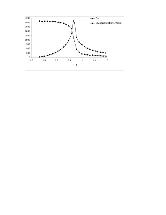
Figure 3: This figure shows the location of the critical temperature, $T_{c}$. In our simulation, it happens at T=2.3 for a $100\times 100$ lattice. Horizontal axis is scaled by $T_{c}=2.269$, the exact value for $T_{c}$. Units are arbitrary.

The above equation was derived based on the fact that the probability distribution of the demons for each layer is Maxwellian. In many respects, the demon acts as a thermometer since it has only one degree of freedom in comparison to the many degrees of freedom of the system with which it exchanges energy. After taking sufficient time steps during which the temperature of the end layers were being monitored by the Metropolis method and that of the mid-layers by the demon method, a stationary temperature gradient begins to set in. To determine it qualitatively, we calculate the “local” temperature with the use of equation (3) for each sub-layer. In figure 1 we have plotted the temperature of sub-layers versus the $x$-coordinates of the layers corresponding to the original lattice for several high and low temperatures. As can be seen, the fluctuations of the temperature profiles about the mean temperature are extremely small. Figure 2 shows variation of the magnetization profile versus the lattice size per spin. These figures clearly show that a steady state in heat transport has set in. It is also worth mentioning that as $T_{m}$ gets closer to the critical temperature, a temperature gradient still persists. To find the critical temperature $T_{c}$ in our system, we did a simulation using a greater size (10000 spins in a $100\times 100$ lattice) and found that the critical temperature is near 2.3 which is very close to the exact result of $2.269$ [6], as shown in figure 3. The exact value for $T_{c}$ has been used throughout the paper for scaling the horizontal axes for all the relevant figures. The heat flux $\bf Q$ is the amount of energy that the hot layer adds to the system and is computed by subtracting the total energy of the hot $(E_{hot})$ and cold $(E_{cold})$ layers per unit area per Monte Carlo step for each $T_{m}$ resulting from individual $T_{h}$ and $T_{l}$. For calculating thermal conductivity we use

$$K(T_{m})=\frac{E_{hot}-E_{cold}}{\frac{\Delta{T}}{\Delta{X}}{A\tau}},$$ (4)

where $A$ is the area which in our 2D model represents the system size in the $y$-direction and $\tau$ is conventionally measured in terms of the Monte Carlo steps per spin. It should be noted that the effects of the mid-layers in the calculation of thermal conductivity are contained in the temperature gradient $\Delta T/\Delta X$ which changes from temperature to temperature.

3 Theoretical considerations

In this section we shall be concerned with an analysis in which we investigate the dependence of heat conductivity on the size of the system and temperature. Our analysis is based on the equilibrium kinetic Ising system and the Green-Kubo relation [7, 8] for heat conductivity according to which

$$K(T,L)=\frac{1}{3K_{\tiny\mbox{B}}T^{2}}\int_{0}^{\infty}dt\int dr\langle{\bf Q}(0,0)\cdot{\bf Q}(r,t)\rangle,$$ (5)

where ${\bf Q}$ is now the instantaneous heat current vector in an assembly of $N$ interacting spins, $T$ is the temperature and the angle brackets, $\langle\cdots\rangle$, indicate equilibrium ensemble average. Definition of $\bf Q$ in terms of the variation of magnetization is an interesting question to which a considerable amount of attention is being paid [10]. It would be useful to note that the integrand in equation (5), as will be discussed below, depends on the size of the system and therefore integration on $r$ has to be done independently.

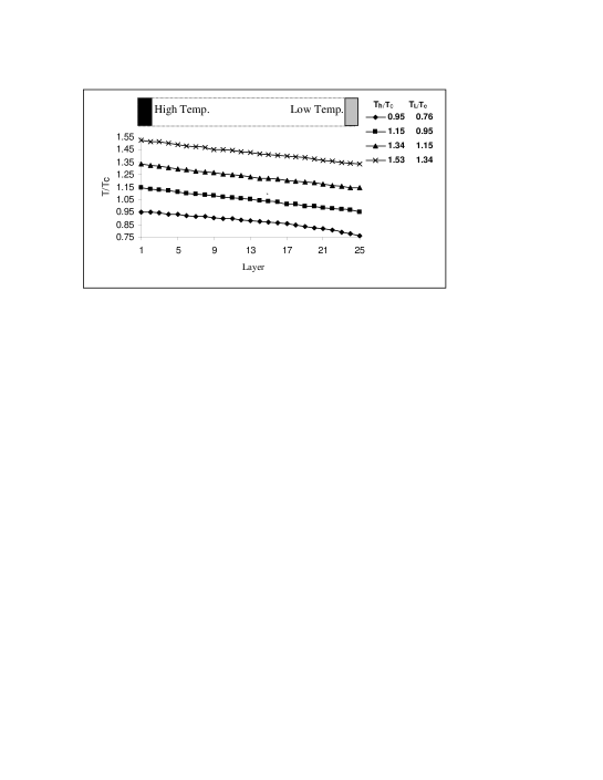
Figure 1: Local temperature profile in a $100\times 100$ Ising lattice with different gradients.

Heat current vectors depend on the rate of change of the direction of spins. Consequently, transferring this change to the direction of temperature gradient is highly dependent on the correlation functions. Also, correlation functions depend on temperature and vanish above $T_{c}$, their values approaching unity around $T_{c}$. In fact, heat transport is the transmission of information by the spins as they flip. In the limit of high temperature, heat transport hardly occurs because both the correlation functions and transmission of the flipping of the spins are small. However, each spin flips independently of the others and takes an amount of energy equal to $\pm 2J$. This means that the size of the system becomes an irrelevant parameter, so that thermal conductivity becomes independent of the size. In view of the above discussion, we estimate the integral as

$$K(T)\sim\frac{J^{2}}{T^{2}},$$ (6)

where $J$ is independent of temperature. In addition, in the limit of low temperature and near $T_{c}$, correlation functions increase in value and transmission of information by the spins being flipped is large whereas in the limit $T\rightarrow 0$ the transmsion would be zero, leading to a zero thermal conductivity. When correlation length is larger than the system size, the boundary of the system influences heat transport since the characteristic wavelength of the system is smaller than the correlation length. We expect thermal conductivity to increase as the system size grows. This increasing regime finally stops when system size becomes greater than the correlation length. In the low temperature limit however, each spin has a small chance of being flipped and near zero takes an amount of energy equal to $\epsilon=8J$ with probability $\exp(-\epsilon/T)$ after a flipping has occurred. Indeed, near $T_{c}$, $\epsilon$ is smaller than $8J$. Summarizing, we may deduce the following formula for thermal conductivity

$$K(T,L)\sim\frac{J^{2}L^{\alpha}\exp(-\epsilon/T)}{T^{2}},$$ (7)

where $\alpha$ is a dimensionless positive quantity that tends to zero in the limit of large system sizes. The dependence of $K$ on $L$ may be better understood in the light of the dependence of specific heat $C_{B}$ on the system size and its relation to thermal conductivity which may be crudely written as $K\sim C_{B}L$. It would be interesting to note that the same results have been reported in [11] for various potential models.

4  Results

A discussion of the results we have obtained from our simulations is now in order. The initial configuration of the 2D system was selected by randomizing square lattices consisting of $N$=1024, 2025, 3247, 4761, 6400, 8100 and 10000 spins. The lattice was layered along the $x$-axis, each layer consisting of 64, 125, $\cdots$ sites respectively and may also consist of 2, 3, or 4 columns of spins in the y direction. A typical configuration includes $100\times 100$ cites consisting of 25 layers, each made of 4 columns of spins. For simplicity, we adopt $J$ as the unit of energy.

Figure 2: Variation of the magnetization profile per spin versus the lattice size for three different temperature gradients with a lattice size of $100\times 100$. The figure in the middle corresponds to the largest temperature gradient and that on the top is a snapshot of a system consisting of $32\times 32$ spins with the same temperature gradient as the figure in the middle. The dark and light points represent opposite spins. Units are arbitrary.

Thermal conductivity in each case for various sizes has a peak around the critical temperature and shows the usual qualitative behavior for many materials [9] (metals and alloys) as shown in figure 4. It can be seen that as temperature decreases, conductivity of the system increases. The reason is that in the limit of low temperature, correlation length for the spins increases and therefore, as soon as a small amount of heat enters from one side, it would be conducted easily through the spins. This means that the coefficient of conductivity becomes large. Also, when temperature approaches that of the critical $(\approx 0.8T_{c})$, $K$ has a maximum. In the limit of high temperature, thermal conductivity is consistent with the $\frac{1}{T^{2}}$ behavior, as we expect from the above theoretical discussion. As a matter of discussion, it should be mentioned that one cannot express thermal conductivity in the Ising system in any quantitative way because we employ a rather simple model and do not know anything about the time and distance between adjacent spins in our Monte Carlo simulations. Therefore, one cannot say much about the unit of thermal conductivity. Equation (7) shows that in the limit of low temperature, $K$ passes through a maximum in the Ising system. We have fitted our simulation data using this equation and obtained $\epsilon=1.45$ for ferromagnetic and $\epsilon=1.47$ for anti-ferromagnetic cases as has been shown in figure 5. It is worth mentioning at this point that the values for $\epsilon$ mentioned above have been obtained using the interval in which thermal conductivity is peaked. Furthermore, in the high temperature limit the correlation length and correlation time are small and the Green-Kubo relation leads to equation (6) which is in good agreement with our simulation results, see figure 6. As can be seen in figures 4 and 6, our calculations are in agreement with both ranges of temperatures. We have also demonstrated, within the context of this model, that for a given temperature gradient, thermal conductivity increases with size as

$$K=cL^{\alpha},$$ (8)

where $\alpha$ is a positive function of temperature and approaches zero at high temperature, as is shown in the table attached to figure 7 which exhibits thermal conductivity decreasing as the lattice size is reduced. This is an interesting behavior and is in agreement with the above discussion on size effects.

In the presence of an external magnetic field $h$, equation (3) would be converted to the following equation

$${T}=\frac{4/d}{\log\left(1+\frac{4/d}{\langle E_{d}(l)\rangle}\right)},$$ (9)

where $d=\frac{2b}{h}$ with $b$ and $d$ being relative prime positive integers and, in the limit of $h\rightarrow 0$, we recover equation (3) as has been described in [4]. In the limit of zero temperature or near the critical temperature, due to the freezing of spins, the demon energy for each layer, $\langle E_{d}\rangle$, would be reduced in such a manner as to result in a zero average. This can be investigated by letting $\langle E_{d}\rangle$ go to zero in equation (9) which will result in unacceptable values for local temperatures. Even in limit $T/T_{c}<2$ we could not obtain good results for temperature gradients, in contrast to higher temperatures where reasonable gradients are obtained similar to those shown in figure 1.

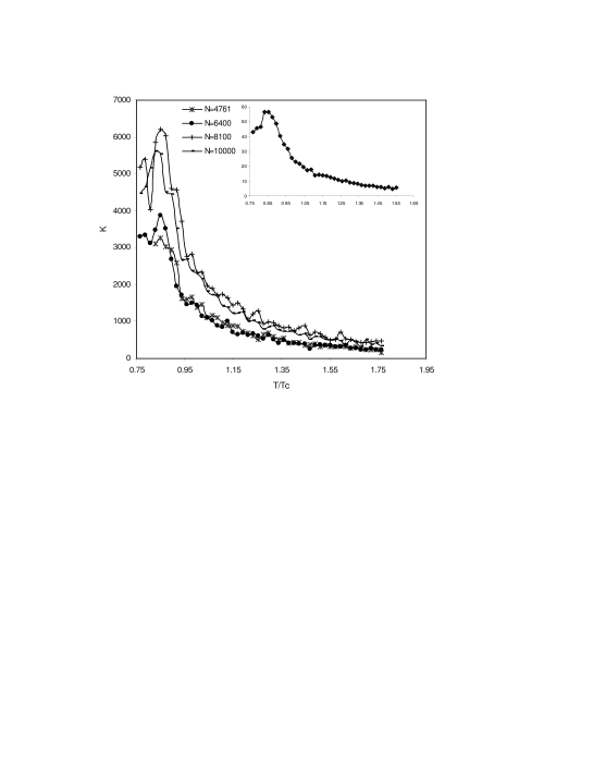
Figure 4: Temperature dependence of thermal conductivity for various system sizes. This figure shows that for temperatures less than $T_{c}$, $K$ increases and passes through a maximum. Afterwards, $K$ would decrease according to equations (6,7). Note that as the system size becomes larger, the peaks representing $T/T_{c}$ approach unity. The insert indicates the same results for a $100\times 100$ antiferromagnetism system. Units are arbitrary.

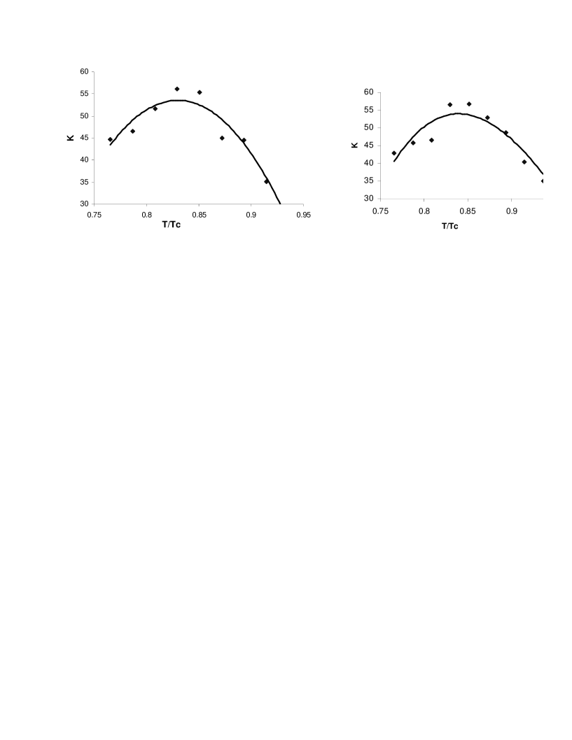
Figure 5: Points showing simulation results for temperatures smaller than $T_{c}$ and around it. The solid line demonstrates the behavior according to equation (7), left, for $J<0$ and right, for $J>0$ with arbitrary units.

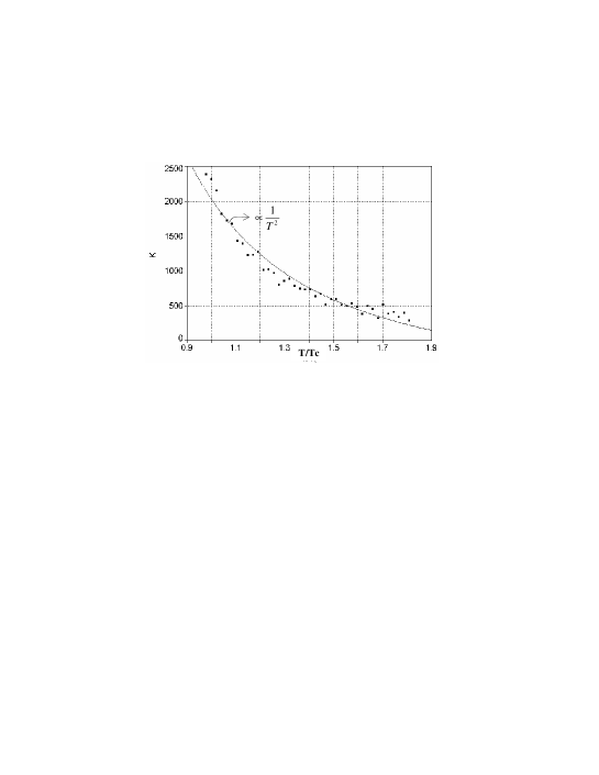
Figure 6: The points present simulation results and the solid line showing theoretical prediction for temperatures above $T_{c}$ according to equation (6) with arbitrary units.

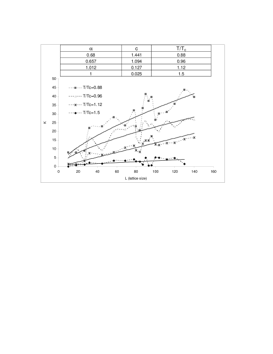
Figure 7: The effect of size on thermal conductivity. $K$ grows from zero exponentially and, as can be seen, decreases with temperature. The table shows how the values of $c$ and $\alpha$ change with temperature in equation (8) with arbitrary units.

5 Conclusions

In spite of its simplicity, the Ising system has been used in a myriad of applications in modelling and simulating various systems. Figures 4 and 7 make it easy to see the size effects becoming important in the small spin systems within the context of the model presented here. These figures illustrate the influence of both the size and temperature effects on thermal conductivity for a simple 2D Ising system. The influence of temperature, however, is not a new subject theoretically. These figures show that thermal conductivity increases when temperature is reduced. On the other hand, figure 7 shows that thermal conductivity would increase exponentially with increasing system size and goes to zero with a decreasing size in any temperature.

Although our study in this paper has been based on a 2D model, the results can be generalized using a 3-dimensional lattice.
Acknowledgement
We would like to thank H. Rafii-Tabar for useful discussions.

References

- [1] P. Nelson, Biological Physics: Energy, Information, Life (W. H. freeman, New York 2003).
- [2] M. Creutz, Ann. Phys. 167 62 (1986).
- [3] R. Harris and M. Grant, Phys. Rev. B 38 9323 (1988).
- [4] S. S. Mak, Phys. Lett. A 196 318 (1995).
- [5] M. P. Allen and D. J. Tidesley, Computer Simulation Of Liquids (Oxford University Press, Oxford, 1987).
- [6] B. M. Mccoy and T. Tsunwu, The two dimensional ising model (Harvard University Press, Cambridge, 1973).
- [7] M. S. Green, J. Chem. Phys. 22 398 (1954).
- [8] R. Kubo, Rep. Prog. Phys. 49 255 (1986).
- [9] C. Kittle, Introduction to solid state physics, 7th edition (Jhon Wiley & Sons, 1996).
- [10] V. Lecomte, Z. Racz and F. V. Wijland, J. Stat. Mech. P02008 (2005).
- [11] S. Lepri, R. Rivi and A. Politi, Phys. Rep. 377 (2003) 1.