Sensitivity, Itinerancy and Chaos in Partly–Synchronized Weighted Networks

Abstract

We present exact results, as well as some illustrative Monte Carlo simulations, concerning a stochastic network with weighted connections in which the fraction of nodes that are dynamically synchronized, $\rho\in\left[0,1\right],$ is a parameter. This allows one to describe from single–node kinetics $(\rho\rightarrow 0)$ to simultaneous updating of all the variables at each time unit $(\rho\rightarrow 1).$ An example of the former limit is the well–known sequential updating of spins in kinetic magnetic models whereas the latter limit is common for updating complex cellular automata. The emergent behavior changes dramatically as $\rho$ is varied. For small values of $\rho,$ we observe relaxation towards one of the attractors and a great sensibility to external stimuli and, for $\rho\geq\rho_{c},$ itinerancy as in heteroclinic paths among attractors; tuning $\rho$ in this regime, the oscillations with time may abruptly change from regular to chaotic and vice versa. We show how these observations, which may be relevant concerning computational strategies, closely resemble some actual situations related to both searching and states of attention in the brain.

PACS: 02.50.Ey; 05.45.Gg; 05.70.Ln; 87.18.Sn; 89.20.-a

1 Introduction and definition of basic model

A dynamic network of many nodes connected by weighted communication lines models a great variety of situations in physics, biology, chemistry and sociology, and it has a wide range of technological applications as well; see, for instance, [1, 2, 3, 4, 5, 6, 7]. Examples of weighted networks are the metabolic and food webs, which connect chains of different intensity, the Internet, the world wide web and other social networks, in which agents may interchange different amounts of information or money, the transport nets, whose connections differ in capacity, number of transits and/or passengers, spin glasses and reaction–diffusion systems, in which diffusion, local rearrangements and reactions may vary the effective ionic interactions, and the immune system, the central nervous system and the brain, e.g., high–level functions in the latter case seem to rely on synaptic changes.

A rather general feature in these systems is that the nodes are not fully synchronized when performing a given task —which may be either a matter of economy or else, perhaps more frequently, a necessary condition for efficient performance. Even though this is as evident as the fact that links are seldom homogeneous, studies of partly synchronized networks are rare. Furthermore, the relevant literature is dispersed, as it was generated in various distant fields, and a broad coherent description is lacking. In particular, related studies often disregard an important general property, namely, that the systems of interest are out of equilibrium. That is, they cannot settle down into an equilibrium state but the network typically keeps wandering in a complex space of fixed points or, in one of the simplest cases, it reaches a nonequilibrium steady state whose nature depends on dynamic details [2]. This results in a complex landscape of emergent properties whose relation with the network details is poorly understood. In this paper, as a new effort aimed at methodizing somewhat the picture, we present some related exact results, together with illustrative Monte Carlo simulations, which apply to a rather general class of partly–synchronized heterogeneous or weighted networks. It follows, as a first application, examples of itinerancy and constructive chaos which mimic recent experimental observations.

Consider a network, with a processor, neuron, spin or, simply, variable at each node, and define the sets of node activities, $\mathbf{\sigma}\equiv\left\{\sigma_{i}\right\},$ and communication line weights, $\mathbf{w}\equiv\left\{w_{ij}\right\},$ where $i,j=1,\ldots,N.$ Each node is acted on by a local field $h_{i}\left(\mathbf{\sigma},\mathbf{w}\right)$ which is induced by the weighted action of the other, $N-1$ nodes. We also define an additional, operational set of binary indexes, $\mathbf{x}=\{x_{i}=0\,\,\mathrm{or}\,\,1\}.$ Time evolution proceeds according to a generalized cellular–automaton strategy. That is, at each time unit, one simultaneously modifies the activity of $n$ variables, $1\leqslant n\leqslant N,$ and the probability of the network state evolves in discrete time, $t,$ according to

$$P_{t+1}(\mathbf{\sigma})=\sum_{\mathbf{\sigma}^{{}^{\prime}}}R\left(\mathbf{\sigma}^{\prime}\mathbf{\rightarrow}\mathbf{\sigma}\right)P_{t}(\mathbf{\sigma}^{\prime})$$ (1)

with the (microscopic) transition rate:

$$R\left(\mathbf{\sigma}\mathbf{\rightarrow}\mathbf{\sigma}^{\prime}\right)=\sum_{\mathbf{x}}p_{n}(\mathbf{x})\prod_{\left\{i|x_{i}=1\right\}}\tilde{\varphi}_{n}\left(\sigma_{i}\rightarrow\sigma_{i}^{\prime}\right)\prod_{\left\{i|x_{i}=0\right\}}\delta_{\sigma_{i},\sigma_{i}^{\prime}}.$$ (2)

Here, $\tilde{\varphi}_{n}\left(\sigma_{i}\rightarrow\sigma_{i}^{\prime}\right)\equiv\varphi\left(\sigma_{i}\rightarrow\sigma_{i}^{\prime}\right)\left[1+\left(\delta_{\sigma_{i}^{\prime},-\sigma_{i}}-1\right)\delta_{n,1}\right]$ is the elementary local rate, $\varphi$ is an arbitrary function of $\beta\sigma_{i}h_{i}$ where $\beta$ is an inverse “temperature” —i.e., a parameter which controls the stochasticity of the process— and, for any set of $n$ sites chosen at random, one has that

$$p_{n}\left(\mathbf{x}\right)=\left(\begin{array}[]{c}N\\ n\end{array}\right)^{-1}\delta\left(\sum_{i}x_{i}-n\right).$$ (3)

This is the natural generalization of two familiar cases: The Glauber sequential updating [2] follows for $n=1,$ so that it is obtained macroscopically in the limit of the minimal dynamic perturbation or $\rho\equiv n/N\rightarrow 0,$ while the above reduces to the Little parallel updating [8, 9] for $n=N,$ i.e., as $\rho\rightarrow 1.$ One may think of many situations whose understanding may benefit from studying the crossover between these two situations. For example, assuming a cell which is stimulated only in the presence of a neuromodulator such as dopamine, the parameter $n$ will correspond to the number of neurons that are modulated each cycle. That is, the other $N-n$ neurons receive no input but maintain memory of the previous state, which has been claimed to be at the basis of working memories [10].

2 Some explicit realizations

For simplicity, and also to have well defined references, we shall represent nodes in the following as binary variables, $\sigma_{i}=\pm 1,$ while $w_{ij}\in\mathbb{R},$ and consider local rates $\varphi\left(\sigma_{i}\rightarrow\sigma_{i}^{\prime}=-\sigma_{i}\right)=\frac{1}{2}\left[1-\sigma_{i}\tanh\left(\beta h_{i}\right)\right],$ which is rather customary as a case that satisfies detailed balance [2]. Notice, however, that, in general, detailed balance is not fulfilled by our basic equation (1) nor by the superposition (2) as far as $n>1.$ Consequently, in general, our system cannot be described by Gibbs ensemble theory. We shall further assume that the fields satisfy

$$h_{i}\left(\mathbf{\sigma},\mathbf{w}\right)=h\left[\mathbf{\pi}\left(\mathbf{\sigma}\right),\mathbf{\xi}_{i}\right].$$ (4)

We are assuming here a set of $M$ given patterns, namely, different realizations of the network set of activities, to be denoted as $\mathbf{\xi}\equiv\left\{\mathbf{\xi}_{i}\right\}$ with $\mathbf{\xi}_{i}\equiv\left\{\xi_{i}^{\mu}=\pm 1;\mu=1,\ldots,M\right\},$ and $\mathbf{\pi}\equiv\left\{\pi^{\mu}\left(\mathbf{\sigma}\right)\right\},$ where the product $\pi^{\mu}\left(\mathbf{\sigma}\right)=N^{-1}\sum_{i}\xi_{i}^{\mu}\sigma_{i}$ measures the overlap of the current state with pattern $\mu.$ For $N\rightarrow\infty$ and finite $M,$ i.e., in the limit $\alpha\equiv M/N\rightarrow 0,$ from (1)–(4), the mesoscopic time–evolution equation

$$\pi_{t+1}^{\mu}\left(\mathbf{\sigma}\right)=\rho N^{-1}\sum_{i}\xi_{i}^{\mu}\tanh\left\{\beta h_{i}\left[\mathbf{\pi}_{t}\left(\mathbf{\sigma}\right),\mathbf{\xi}_{i}\right]\right\}+\left(1-\rho\right)\pi_{t}^{\mu}\left(\mathbf{\sigma}\right)$$ (5)

follows for any $\mu.$ The details of the derivation, as well as some possible generalizations of this result, will be published elsewhere [11].

One of the simplest realizations of the above is the Hopfield network [12, 13, 14]. In this case, the communication line weights are heterogeneous but fixed according to the Hebb (learning) prescription $w_{ij}=N^{-1}\sum_{\mu}\xi_{i}^{\mu}\xi_{j}^{\mu},$ and the local fields are $h_{i}\left(\mathbf{\sigma},\mathbf{w}\right)=\sum_{j\neq i}w_{ij}\sigma_{j}.$ These choices satisfy condition (4) which also holds for other non–linear learning rules; in any case, one may easily generalize (5) to include other interesting cases (see, for instance, [15]) which do not precisely conform to (4). The original Hopfield model evolves by Glauber processes, namely, by attempting a single variable change, $\sigma_{i}\rightarrow-\sigma_{i},$ at each unit time —e.g., the Monte Carlo step— with probability $\varphi\left(\beta\sigma_{i}h_{i}\right).$ The symmetry $w_{ij}=w_{ji}$ and detailed balance then guarantee asymptotic convergence to equilibrium, i.e., $P_{t\rightarrow\infty}\left(\mathbf{\sigma}\right)\propto\exp\left(\beta\sum_{i}h_{i}\sigma_{i}\right).$

Computational efficiency has sometimes motivated to induce time evolution of the Hopfield network by the Little strategy, i.e., $\rho\rightarrow 1$ in our formulation. This is known to drive the system to a full nonequilibrium situation, in general [16]. The local rule and other details of dynamics are then essential in determining the emergent behavior. Not only the time evolution may vary but also the nature of the resulting asymptotic state, perhaps including morphology, phase diagram, universality class, etc.; see Refs.[2, 17, 18] for some outstanding examples of this assertion.

For completeness, we mention that the Hopfield network, i.e., $\rho\rightarrow 0$ will also correspond, in general, to a nonequilibrium situation when implemented (unlike in the original proposal [12]) with asymmetric or time–evolving weights or with a dynamic rule lacking detailed balance. There is some chance that an effective Hamiltonian [19], such that $P_{t\rightarrow\infty}\left(\mathbf{\sigma}\right)\propto\exp\left(H_{\mathrm{eff}}\right),$ can then be defined, however. When this is the case, one may often apply equilibrium methods, with the result of relatively simple emergent properties [20, 21].

Concerning our proposal (5), we first mention that, assuming fields that conform to the Hebb prescription with static weights, the Hopfield property of associative memory is recovered for $\rho\rightarrow 0,$ as expected. That is, for high enough $\beta$ (which means below certain stochasticity) the patterns $\mathbf{\xi}$ may be attractors of dynamics. Consequently, an initial state resembling one of the patterns, e.g., a degraded picture will converge towards the original one, which mimics simple recognition [13, 14]. We checked too that, in agreement with some previous indications [22], implementing the Hopfield–Hebb network with $\rho>0$ produces the behavior that characterizes the familiar case $\rho\rightarrow 0,$ including associative memory, even though equilibrium is precluded, e.g., in general, no effective Hamiltonian is predicted to exist for any $\rho>0$ [16]. Excluding these Hopfield–Hebb versions, our model exhibits a complex behavior which depends dramatically on the value of $\rho.$ This is a consequence of changes with $\rho$ in the stability associated with (5), as we show next.

3 Some main results

The local fields may be determined according to various criteria, depending on the specific application of interest. That is, one may investigate the consequences of equation (5) and associated stability for different relations between the fields and the weights $w_{ij}$ and between these and other network properties.

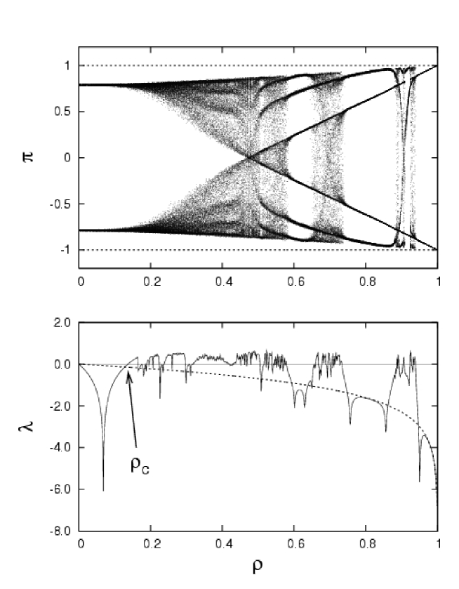
Figure 1: Evidence for critical transitions from regular to chaotic behavior as the synchronization parameter $\rho=n/N$ is varied. Top graph: Monte Carlo results for depressing fluctuations with $\Phi=1/2.$ This shows the dependence on $\rho$ of the stationary overlap between the activity and a single (randomly generated) pattern for $N=3600$ variables, and inverse “temperature” $\beta=20.$ The dashed line is for the standard Hopfield–Hebb case, $\Phi=-1.$ Bottom graph: The dependence on $\rho$ of the Lyapunov exponent, as obtained analytically from the saddle–point solution, for the same case as above (solid irregular line) and for $\Phi=-1$ (dashed line). This graph also shows the value $\rho=\rho_{c},$ i.e., the minimum degree of synchronization needed to observe chaotic behavior, and the line $\lambda=0$ for reference purposses.

We shall be mostly concerned in the rest of this paper with a specific neural automaton as a working example. In this case, the above assumption of static line weights happens to be rather unrealistic. As a matter of fact, one is eager to admit, concerning different contexts, that the communication line weights may change with the nodes activity, and even that they may loose some competence after a time interval of heavy work. This seems confirmed in the case of the brain where the transmission of information and many computations are strongly correlated with activity–induced fast fluctuations of the synaptic intensities, namely, our $w_{ij}$’s [23, 24]. Furthermore, assuming the experimental observation that synaptic changes may induce depression [25] seems to have important consequences [26, 27, 21]. That is, a repeated presynaptic activation may decrease the neurotransmitter release, which will depress the postsynaptic response and, in turn, affect noticeably the system behavior. For concreteness, motivated by these facts, we shall adopt here the proposal in Refs.[21, 28]. This amounts to assume a simple generalization of the Hebb prescription which is in accordance with condition (4), namely,

$$w_{ij}=\left[1-\left(1+\Phi\right)q\left(\mathbf{\pi}\right)\right]N^{-1}\sum_{\mu=1}^{M}\xi_{i}^{\mu}\xi_{j}^{\mu},$$ (6)

where $q\left(\mathbf{\pi}\right)\equiv\left(1+\alpha\right)\sum_{\mu}\pi^{\mu}\left(\mathbf{\sigma}\right)^{2}$ depends on the set of stored patterns. The Hopfield case discussed above is recovered for $\Phi=-1,$ while other values of this parameter correspond to fluctuations which induce depression of synapses by a factor $-\Phi$ on the average.

The choice (6) happens to importantly modify the network behavior, even for a single stored pattern, $M=1.$ The stationary, $t\rightarrow\infty$ solution of (5) is then $\pi_{\infty}=F\left(\pi_{\infty};\rho,\Phi\right)$ with

$$F\left(\pi;\rho,\Phi\right)\equiv\rho\tanh\left\{\beta\pi\left[1-\left(1+\Phi\right)\pi^{2}\right]\right\}+\left(1-\rho\right)\pi,$$ (7)

and local stability requires that $\left|\partial F\left(\pi;\rho,\Phi\right)/\partial\pi\right|<1.$ The fixed point is therefore $\pi_{\infty}=\tanh\left\{\beta\pi_{\infty}\left[1-\left(1+\Phi\right)\pi_{\infty}^{2}\right]\right\},$ independent of $\rho,$ while stability crucially depends on $\rho.$ The limiting condition $\left.\partial F\left(\pi;\rho,\Phi\right)/\partial\pi\right|_{\pi_{\infty}}=1$ corresponds to a steady–state bifurcation. This implies for $\pi_{\infty}=0$ that $\beta<\beta_{c}=1,$ independent of both $\rho$ and $\Phi.$ Non–trivial solutions $\pi_{\infty}\neq 0$ in this case require that $\Phi>-4/3,$ which includes the Hopfield case. The other limiting condition $\left.\partial F\left(\pi;\rho,\Phi\right)/\partial\pi\right|_{\pi_{\infty}}=-1$ corresponds to a period doubling bifurcation. It follows from this that local stability requires $\rho<\rho_{c}$ with

$$\rho_{c}=2\left\{3\beta\pi_{\infty}^{2}\left[\left(\Phi+{\textstyle{4\over 3}}\right)-\left(1+\Phi\right)\pi_{\infty}^{2}\right]-\beta+1\right\}^{-1}.$$ (8)

It is to be remarked that this condition cannot be fulfilled in the Hopfield, $\Phi=-1$ case, for which one obtains from (8) the nonsense solution $\rho_{c}\geq 2.$

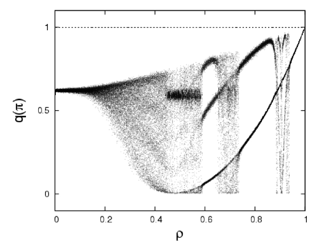
Figure 2: The chaotic behavior in figure 1 occurs also as the number of patterns is increased. This graph shows the dependence on the synchronization parameter $\rho$ of the steady–state value of the order parameter $q\left(\mathbf{\pi}\right)\equiv\left(1+\alpha\right)\sum_{\mu}\pi^{\mu}\left(\mathbf{\sigma}\right)^{2}.$ The behavior shown here —which follows indistinctly from the analytical solution or from Monte Carlo simulations— is for $M=20$ stored (randomly generated) patterns, $N=3600,$ $\beta=20$ and $\Phi=1/2.$ The dashed, horizontal line $q=1$ is for the Hopfield case, $\Phi=-1;$ this illustrates that, except for scaling of the relaxation time, the value of $\rho$ is then irrelevant.

The resulting behavior is illustrated in figure 1. This shows, for $M=1,$ the onset of chaos at $\rho=\rho_{c}$ in the saddle–point map (5) and, accurately fitting this, in Monte Carlo simulations. The behavior shown in the top graph of figure 1, which is for $\Phi=\frac{1}{2},$ is likely to characterize any $\Phi\neq-1$ as well. This behavior does not occur for the singular Hopfield case with static synapses, for which the stability of $\mathbf{\pi}$ is independent of $\rho.$ The bottom graph in figure 1 illustrates that one has for $\rho>\rho_{c}$ regimes of regular oscillations among the attractors (i.e., the given pattern and its “negative” in this case with $M=1)$ which are eventually interrupted as one varies $\rho,$ even slightly, by eventual chaotic jumping.

The critical value of the synchronization parameter for the emergence of chaos, due to local instabilities around the steady $\pi$ solution may be estimated in figure 1 as $\rho_{c}=0.137$ for $M=1.$ This is precisely the value that one obtains from equation (8) for $\beta=20$, $\pi=0.788$ and $\Phi=\frac{1}{2}.$

Figure 2 confirms that this behavior occurs also for $M>>1$ stored patterns, and figure 3 shows the detail during the stationary part of typical runs for representative values of $\rho.$ In particular, figure 3 illustrates qualitatively–different types of time series our model exhibits, namely, from bottom to top: (i) convergence towards one of the attractors —in fact, to one of the antipatterns— for $\rho<\rho_{c};$ (ii) chaos, i.e., fully irregular behavior with a positive Lyapunov exponent for $\rho>\rho_{c};$ (iii) a perfectly regular oscillation between one of the attractors and its negative for $\rho>\rho_{c};$ (iv) onset of chaotic oscillations as $\rho$ is increased somewhat; and (v) very rapid and completely ordered and periodic oscillations between one pattern and its antipattern when all the nodes evolve synchronized with each other at each time step. The cases (ii) and, less markedly, (iv) are nice examples of instability–induced switching phenomena. That is, as suggested also in experiments on biological systems (see next section), the network describes heteroclinic paths among the stored patterns, remaining for different time intervals in the neighborhood of different attractors, the choice of attractor being at random.

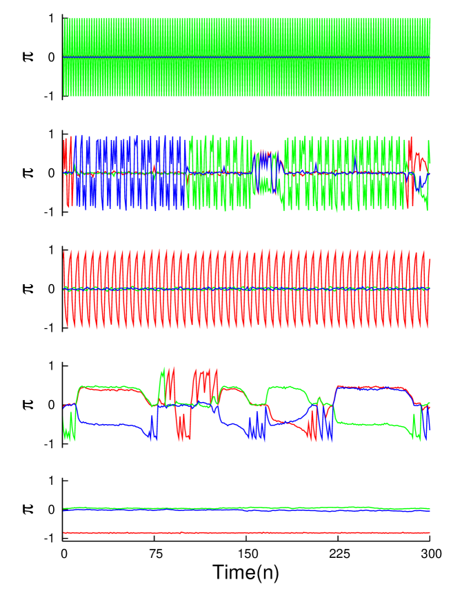
Figure 3: The overlap as a function of time (in units of $n$ MC trials) after a transient time $t=1920n,$ for $N=1600,$ $\beta=20,$ $\Phi=0.4$ and $M=3$ uncorrelated patterns. It follows in this case that $\rho_{c}=0.085.$ Different graphs are for increasing values of $\rho$ from bottom to top, namely, for $\rho=0.08,$ 0.50, 0.65, 0.92 and 1.00, respectively.

4 Discussion

In summary, we report in this paper on a class of homogeneous or weighted networks in which the density, $\rho,$ or the number of variables that are synchronously updated at a time may be varied. This is remotely related to block–dynamics, block–sequential, and associated algorithms [29, 30], which aim at more efficient computations, and it generalizes some previous proposals [31, 22, 32]. We describe in detail the behavior of a particular realization of the class, namely, a neural automaton which is motivated by recent neurobiological experiments and related theoretical analysis. Different realizations of the class correspond to different choices of the local fields $h\left(\mathbf{\pi},\mathbf{\xi}\right)$ that act upon the stochastic variables at the (neural) nodes. For certain values of these fields, which amount to fix the (synaptic) connections at some constant values, e.g., according to the Hebb prescription, one recovers the equilibrium Hopfield network. The parameter $\rho$ is then irrelevant concerning most of the system properties. Our model also admits simple extensions, corresponding to other values of the local fields, that one may characterize by a complex effective temperature [2, 21].

The Hopfield picture has severe limitations concerning its practical usefulness [14], and some of these limitations may be overcome by producing a full nonequilibrium condition. It is sensible to expect that $\rho$ will then transform into a relevant parameter. This is, in fact, the situation in [31] which deals with a modification of the Hebb prescription which includes multiple interactions, random dilution and a Gaussian noise. This implies a choice for the fields that even precludes the existence of an effective temperature, and chaotic neural activity ensues. Our biologically motivated choice, namely, Hopfield local fields with the simple prescription (6), which is interpreted as a consequence of depressing synaptic fluctuations, induces a full nonequilibrium condition —even for $\rho\rightarrow 0.$ In this limit, the system was recently shown to exhibit enhancement of the network sensitivity to external stimuli [21]. This happens to be a feature of the system for any $\rho.$ This interesting behavior, which we illustrate in figure 4, corresponds to a type of instability which is known to occur in nature, as discussed below. This is associated here to a modification of the topology of the space of fixed points due to the action of the involved $\Phi$–controlled noise.

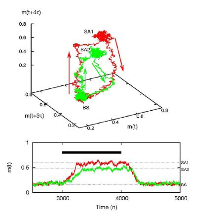
Figure 4: Itinerancy induced by an external stimulus. This shows the mean firing rate as a function of time (bottom graph) and as a phase space three–dimensional trajectory (top graph) when the system is perturbed as explained in the main text. The situation here closely resembles the experimental observation concerning odor responses in figures 2 and 4 in Ref. [33]. The graphs here correspond to the Monte Carlo simulation of our system with $N=1600,$ $T=0.25,$ $\Phi=0.45,$ $\rho=3/64<\rho_{c},$ and six stored patterns. The time unit corresponds to $n$ trials. Performing the top graph required a standard false–neighbor method which indicated an embedding dimension [34] of 5. The involved time delay is $\tau=20n$ MC trials.

Figure 4 is a model remake of experiments on the odor response of the (projection) neurons in the locust antennal lobe [33]. Our simulation illustrates two time series (with different colors) for the mean firing rate, $m=\frac{1}{2N}\sum_{i}\left(1+\sigma_{i}\right),$ in a system with six stored patterns which is exposed to two different stimuli of the same intensity and duration (between 3000 and 4000 time steps —each step corresponding here to $n$ trials). Each pattern consists of a string of $N$ binary variables; three of them are generated at random with, respectively, 40%, 50% and 60% of the variables set equal to 1 (the rest are set equal to $-1),$ while the other three have the 1s at the first 70%, 50% and 20% positions in the string, respectively. The bottom graph shows with horizontal lines the baseline activity without stimulus (BS) and the network activity level in the presence of the stimulus $\mu=1$ (SA1) and $\mu=2$ (SA2), which correspond to two of the random stored patterns.

The conclusion is that the stimulus destabilizes the system activity as in the laboratory experiments. Note, however, that this occurs for $\rho<\rho_{c},$ i.e., in the absence of chaotic behavior. As a matter of fact, the behavior in figure 4 will also be exhibited in the limit $\rho\rightarrow 0$ which does not show any irregular behavior [21].

On the other hand, the suggestion that fluctuating connections may induce fractal or strange attractors as far as $\rho>0$ [32, 28] is confirmed here. As illustrated in figure 3, our system may exhibit both static and kind of dynamic associative memory in this case. That is, the network state either will go to one of the attractors (corresponding to one of the given patterns stored in the connecting synapses) or else, for $\rho\geq\rho_{c},$ will forever remain visiting several or perhaps all the possible attractors. Furthermore, the inspection rounds may abruptly become irregular and even chaotic as the density of synchronized neurons varies slightly. It follows, in particular, that the most interesting, oscillatory behavior requires synchronization of a minimum of variables, and also that occurring chaotic jumps between attractors requires some careful tuning of $\rho.$ In fact, as illustrated in the bottom graph of figure 1, once the critical condition $\rho>\rho_{c}$ is fulfilled a complex situation ensues where it seems difficult to predict the resulting behavior for slight variations of $\rho.$

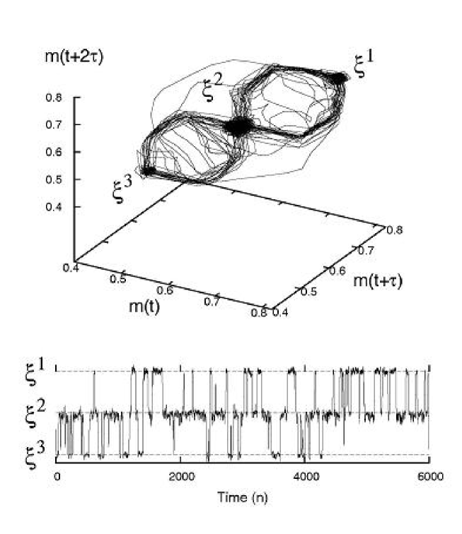
Figure 5: Instability and switching among the attractors as in a state of attention induced by chaos. The mean firing rate as a function of time (bottom graph) and as a trajectory in a three–dimensional phase space (top graph) correspond here to a simulation with $N=1600,$ $T=0.006,$ $\Phi=\frac{1}{2},$ $\rho=123/320>\rho_{c}$ in a chaotic window, and three stored patterns denoted $\xi^{\mu}.$ The top graph involves an embedded dimension of 5 and a time delay $\tau=5n$ MC trials.

The chaotic behavior is further illustrated in figure 5. This shows trajectories among the three stored patterns, namely, $\mathbf{\xi}^{1},$ $\mathbf{\xi}^{2}$ and $\mathbf{\xi}^{3},$ $\mathbf{\xi}^{\mu}=\left\{\xi_{i}^{\mu};i=1,\ldots,N\right\}.$ These are designed, respectively, as a homogeneous string of 1s, a string with the first 50% positions set to 1 and the rest to $-1,$ and as a string with only the first 20% positions set to 1. We observe many jumps between two close (more correlated) patterns and, eventually, a jump to the most distant pattern.

It seems sensible to comment on this behavior at the light of the growing evidence of chaotic behavior in the nervous system [35, 36]. We have shown (e.g., figure 4) that chaos is not needed to have efficient adaptation to a changing environment. However, one may argue [35], for instance, that the instability inherent to chaotic motions facilitates this and, in particular, the system ability to move to any pattern at any time. This behavior, which has been described for the activity of the olfactory bulb and other cases, is nicely illustrated in figures 3 and 5. Our network thus mimics the observed correlation between chaotic neuron activity and states of attention in the brain, as well as other cases of constructive chaos in biology [37, 38, 39, 40].

Chaos has been reported in other interesting networks (e.g., Ref. [41]) but, to our knowledge, never in such a general setting as here. As a matter of fact, the present model allows for some natural generalizations [11] and, in particular, suggests a great interest for a more detailed study of the apparently unpredictable behavior it exhibits for $\rho>\rho_{c}.$ This teaches us that varying $\rho$ is a simple method to control chaos in networks, and that this may also help in determining efficient computation strategies [42, 43]. Concerning the latter, the model behavior may be relevant, for instance, when judging on the best procedure for specific data mining and for the control of different activities on a multiprocessor system [44], and deciding on whether to implement sequential or parallel programming in some extreme cases [45]. Our findings here may also help one in interpreting recent experimental evidence of parallel processing in laminar neocortex microcircuits [46, 47]. That is, a comparison between the model behavior and experimental results may shed light on the dynamics of these circuits and their mutual interactions.

We thank I. Erchova, P.L. Garrido and H.J. Kappen for very useful comments. This work was financed by FEDER, MEyC and JA under projects FIS2005-00791 and FQM–165. JMC also acknowledges financial support from the EPSRC-funded COLAMN project Ref. EP/CO 10841/1.

References

- [1] G. Manganaro et al. , “Cellular Neural Networks”, Springer, Berlin 1999.
- [2] J. Marro and R. Dickman, “Nonequilibrium Phase Transitions in Lattice Models”, Cambridge University Press, Cambridge 1999.
- [3] M.E.J. Newman, SIAM Reviews 45, 167 (2003); ibid, Phys. Rev. E 70, 056131 (2004)
- [4] A. Barrat et al., Proc. Natl. Acad. Sci. USA 101, 3747 (2004)
- [5] P.L. Garrido et al., eds., “Modeling Cooperative Behavior in the Social Sciences”, AIP Conf. Proc., Vol. 779, American Institute of Physics, N.Y. 2005.
- [6] D. Armbruster et al. ”Networks of Interacting Machines”, World Sci., Singapore 2005.
- [7] S. Valverde and R.V. Solé, Europhys. Lett., in press; preprint arXiv:physics/0602005.
- [8] W.A. Little, Math. Biosci. 19, 101 (1974)
- [9] B. Chopard and M. Droz, “Cellular Automata Modeling of Physical Systems”, Cambridge University Press, Cambridge 1998.
- [10] A.V. Egorov et al., Nature 420, 173 (2000)
- [11] J. M. Cortes et al., to be published.
- [12] J.J. Hopfield, Proc. Nat. Acad. Sci. USA 79, 2554 (1982)
- [13] D.J. Amit, “Modeling Brain Function”, Cambridge University Press, Cambridge 1989.
- [14] P. Peretto, “An Introduction to the Modeling of Neural Networks”, Cambridge University Press, Cambridge, 1992.
- [15] J.L. van Hemmen, Phys. Rev. A 36, 1959 (1987)
- [16] G. Grinstein et al., Phys. Rev. Lett. 55, 2527 (1985)
- [17] G. Ódor, Rev. Mod. Phys. 76, 663 (2004)
- [18] J. Marro et al., Phys. Rev. E 72, 026103 (2005)
- [19] P.L. Garrido and J. Marro, Phys. Rev. Lett. 62, 1929 (1989)
- [20] J.J. Torres et al., J. Phys. A: Math. Gen. 30, 7801 (1997)
- [21] J.M. Cortes et al., Neural Comp., 18, 614 (2006)
- [22] A.V.M. Herz and C.M. Marcus, Phys. Rev. E 47, 2155 (1993)
- [23] D. Ferster, Science 273, 1812 (1996)
- [24] L.F. Abbott and W.G. Regehr, Nature 431, 796 (2004)
- [25] M.V. Tsodyks et al. Neural Comp. 10, 821 (1998); A.M. Thomson et al. Philos. Trans. R. Soc. Lond. B Biol. Sci. 357, 1781 (2002)
- [26] L. Pantic et al. Neural Comp. 14, 2903 (2002)
- [27] D. Bibitchkov et al., Network: Comp. Neural Syst. 13, 115 (2002)
- [28] J. Marro et al., submitted (2006)
- [29] F. Martinelli, Lecture Notes in Mathematics 1717, 93 (2000)
- [30] D. Randall and P. Tetali, J. Math. Phys. 41, 1598 (2000)
- [31] L. Wang and J. Ross, Phys. Rev. A 44, R2259 (1991)
- [32] J.M. Cortes et al., Biosystems, in press; q-bio.NC/0510003 (2006)
- [33] O. Mazor and G. Laurent, Neuron 48, 661 (2005)
- [34] J.P. Eckmann and D. Ruelle, Rev. Mod. Phys.
- [35] H. Korn and P. Faure, C. R. Biologies 326, 787 (2003)
- [36] L. Glass, in “Handbook of Brain Theory and Neural Networks”, M.A. Arbib Ed., pp. 205, MIT Press, 2003.
- [37] W. J. Freeman, Biol. Cybern. 56, 139 (1987)
- [38] D. Hansel and H. Sompolinsky, Phys. Rev. Lett. 68, 718 (1992); ibid, J. Comput. Neurosci. 3, 7 (1996)
- [39] G. Laurent et al. Annu. Rev. Neurosci. 24, 263 (2001)
- [40] P. Ashwin and M. Timme, Nature 436, 36 (2005)
- [41] D.R.C. Dominguez and W.K. Theumann, J. Phys. A: Math. Gen. 30, 1403 (1997)
- [42] R. Legenstein and W. Maass, in “New Diractions in Statistical Signal Processing: From Systems to Brain”, S. Haykin et al. editors, The MIT Press, 2005.
- [43] N. Bertschinger and T. Natschläger, Neural Comp. 16, 1413 (2004)
- [44] A. Mueller, Technical report (unpublished), College Park, MD, USA
- [45] P.T. Tosic, in “Conf. Computing Frontiers”, edited by S. Vassiliadis et al. eds., pp.488–502, ACM, Italy 2004.
- [46] E.M. Callaway, Annu. Rev. Neurosci. 21, 47 (1998)
- [47] A.M. Thomson and A. P. Bannister, Cerebral Cortex 13, 5 (2003)