A reevaluation of the coupling to a bosonic mode of the charge carriers in (Bi,Pb)₂Sr₂CaCu₂O_8+δ at the antinodal point

Abstract

Angle-resolved photoemission spectroscopy (ARPES) is used to study the spectral function of the optimally doped high-T_c superconductor (Bi,Pb)₂Sr₂CaCu₂O_8+δ in the vicinity of the antinodal point in the superconducting state. Using a parameterized self-energy function, it was possible to describe both the coherent and the incoherent spectral weight of the bonding and the antibonding band. The renormalization effects can be assigned to a very strong coupling to the magnetic resonance mode and at higher energies to a bandwidth renormalization by a factor of two, probably caused by a coupling to a continuum. The present reevaluation of the ARPES data allows to come to a more reliable determination of the value of the coupling strength of the charge carriers to the mode. The experimental results for the dressing of the charge carriers are compared to theoretical models.

I Introduction

The dressing of the charge carriers in high-T_c superconductors (HTSCs) is still one of the most exciting topics in solid state physics. The HTSCs are a paradigm for the transition of a correlated system from an insulating to a metallic state. The dressing of the charge carriers in HTSCs is likely caused by the same interaction that gives rise to the superconductivity, hence the understanding of the quasiparticle self-energy may help to understand the origin of the mechanism of high-T_c superconductivity. The dressing can be studied by various experimental methods but angle-resolved photoemission spectroscopy is the only method which gives a quantitative information on the momentum dependence of those renormalization effects. In HTSCs there are two important regions on the Fermi surface: the nodal region, where the diagonal of the Brillouin zone cuts the Fermi surface and where the $d-$wave superconducting order parameter changes sign. This region mostly contributes to the transport properties, particularly in the underdoped region, where a pseudogap opens up, squeezing the Fermi surface to a region near the nodes. The other (antinodal) region is one where the edge of the Brillouin zone cuts the Fermi surface. In this region, the order parameter in hole doped superconductors has its maximum. This region is therefore mostly relevant for the studies of the superconducting properties. There are numerous ARPES studies on the renormalization effects near the nodal point,Damascelli ; Campuzano ; Fink but only a few studies are concentrated at the antinodal point Dessau ; Norman1 ; Kaminski ; Sato ; Kim ; Gromko .

In the bilayer systems the study of the antinodal point is complicated by the bilayer splitting, which could not be resolved for 15 years. On the other hand, only in the bilayer system of the Bi-HTSC family the entire superconducting region from underdoped (UD) via optimally doped (OP) to overdoped (OD) can be studied. In the superconducting state a well pronounced peak-dip-hump structure has been detected Dessau ; Norman1 . This structure was originally explained Norman1 ; ABCHU solely in terms of a coupling to a bosonic mode, similar to the McMillan-Rowell explanation of the tunnelling spectra in conventional superconductorsMcMillan69 . Later on, it was established that this peak-dip-hump structure is partially caused by the bilayer splitting Kordyuk5 ; Borisenko3 . By varying the photon energy h$\upsilon$ in the ARPES experiments, and exploiting the different energy dependence of the matrix elements for the excitations from the bonding and the antibonding bands, it became possible to separate the two bands Kim ; Kordyuk5 ; Borisenko3 ; Bansil ; Fujimori and to extract the full energy- and momentum-dependent spectral weight separately in each of the bands. This procedure allowed the authors of Refs. Kordyuk5, ; Borisenko3, to find the intrinsic peak-dip-hump structure, and to demonstrate that the strength of this intrinsic effect is doping-dependent, and decreases in going from UD to OD materials.

An important characteristic of the interaction between fermionic and bosonic excitations is the energy-dependent, dimensionless coupling $\lambda_{E}$. In theories where the fermionic self-energy depends on energy, $E$, much stronger than on the momentum $k-k_{F}$, this dimensionless coupling is related to the self-energy via $\Sigma(E)=-E\lambda_{E}$. It is also relevant whether the measurements are performed in the normal or in the superconducting state. We will label the corresponding couplings as $\lambda_{n,E}$ and $\lambda_{sc,E}$, respectively.

If the normal state is a Fermi liquid, $\lambda_{n,E=0}=\lambda_{n}$ is finite, and is often called a dimensionless coupling constant. It determines the mass renormalization of the fermionic quasiparticles via $m^{*}=m(1+\lambda_{n})$. The coupling constant can, in principle, be extracted from ARPES measurements of the quasiparticle dispersion in the normal state at the lowest energies, however this procedure requires one to know both $k_{F}$ and the bare mass, $m$. In previous analysis Kim , the mass, $m$, was extracted from a tight-binding model with parameters derived from a fit of the Fermi surface and from the quasiparticle dispersion measured along the nodal direction Kordyuk1 ; Kordyuk2 . The analysis of the experimental data in the antinodal region yielded $\lambda_{n}\sim 1.5$ both in UD and OD materials. This result should be contrasted with values Kordyuk6 of $\lambda_{n}\leq 1$ at the nodal point. It is consistent with expectations as for non rotationally-invariant systems the coupling $\lambda_{n}$ depends on the position on the Fermi surface.

In the superconducting state, the measured quasiparticle energy in the antinodal region is bounded by the superconducting gap, $\Delta$, and it becomes an issue at which energy one extracts the coupling $\lambda_{sc,E}$ from the data. In previous analysis, the coupling was extracted from the self-energy measured at $|E|\geq\Delta$. This coupling $\lambda_{sc,\Delta}$ turns out to be larger than $\lambda_{n}$, and it also rapidly increases from OD to UD samples ($\lambda_{sc,\Delta}\sim 8$ for dopant concentration $0.12$).

In this communication we extend our previous analysis of the antinodal self-energy in the superconducting state Kim and show how one can extract the coupling at zero frequency $\lambda_{sc,E=0}\equiv\lambda_{sc}$ from the ARPES data. We find that $\lambda_{sc}$ is smaller than $\lambda_{sc,\Delta}$ and within a certain model is also smaller than the normal state coupling $\lambda_{n}$, in agreement with earlier calculations Chubukov . We show that the large value of $\lambda_{sc,\Delta}$ and its strong doping dependence are at least partially due to the fact that the fermionic self-energy in a superconductor actually diverges at $|E|=\Delta+\Omega_{0}$, where $\Omega_{0}$ is the energy of the bosonic mode. If the bosonic mode is the spin resonance peak, its energy decreases with decreasing doping. Then $|E|=\Delta$ and $|E|=\Delta+\Omega_{0}$ come closer to each other in the UD regime, and $\lambda_{sc,\Delta}$ strongly increases. This is consistent with the analysis in Ref. Kim, .

Our present analysis is based on the measurements of the quasiparticle spectral function in the antinodal region of the high-T_c superconductor (Bi,Pb)₂Sr₂CaCu₂O_8+δ (BiPb2212) in the superconducting state. We go beyond a previous ARPES study which has analyzed the energy dependence of the spectral weight just at the $(\pi,0)$ point Norman , and study the whole antinodal region. We interpret our results in the superconducting state in terms of model self-energy function which is composed of two terms. The first and dominant term is due to a strong coupling of the charge carriers to a single bosonic mode. The second term describes a band renormalization at higher energies and is assumed to have a Fermi-liquid form. We extract both couplings from the fits to the data. We used two models for electron-boson coupling. The first model is a one-mode model for an interaction with an Einstein boson, which is assumed to be independent on fermions. Second is a collective mode model, in which the bosonic spectrum in the normal state is rather flat and incoherent, but splits into a mode and into gapped continuum in the superconducting state due to the feedback effect from the pairing. This second model is appropriate if the boson is a spin collective mode of fermions. We obtain a rather good agreement between the parameters derived from the analysis of the experimental data using the model self-energy function and the calculated values using the collective mode model. This yields a strong indication that the dominant part of the renormalization of the fermionic dispersion is due to a coupling of collective spin excitations.

The paper is organized as follows. In Sec. II we review the two fermion-boson models in the normal and the superconducting state. The experimental setup is discussed in Sec. III. In Sec. IV we present the experimental results together with the data analysis. In Sec. V we discuss the results and compare them with other renormalization effects studied by ARPES in solid state physics. The conclusions of our study are presented in Sec. VI.

II The fermion-boson models

The coupling of the charge carriers to bosonic excitations is the minimum model to understand the spectral function of the HTSCs at the antinodal point. We start with an assumption that the Fermi energy $E_{F}$ is much larger than the mode energy $\Omega_{0}$. The validity of this assumption for very underdoped cuprates has been questioned recently KShen ; Roesch because there the bandwidth is strongly reduced due to correlation effects associated with Mott physics. Here we restrict our analysis to near-optimally doped cuprates for which there is little doubt that $E_{F}\gg\Omega_{0}$ since $E_{F}$ $\sim$ 1 eV in this case.

Both fermion-boson models have been discussed earlier in the literature Norman ; Schrieffer ; Scalapino ; Eschrig ; ABCHU ; Devereaux . We review them here again in order to specify the parameters which can be derived from ARPES. We also present several new results for the collective excitations model.

The dynamics of an electron in an interacting system can be described by a Green’s function Mahan

$$G(E,k)=\frac{1}{E-\epsilon_{k}-\Sigma(E,k)}.$$ (1)

where $\Sigma(E,k)$=$\Sigma^{\prime}(E,k)$+i$\Sigma^{\prime\prime}(E,k)$ is the complex self-energy function which contains the information on the fermion-boson interaction, and $\epsilon_{k}$ is the bare quasiparticle dispersion. Near the Fermi surface $\epsilon_{k}=v_{F}(k-k_{F})$, where $v_{F}=k_{F}/m$, and $m$ is the bare mass. It is customary to use the tight-binding form for $\epsilon_{k}$.

ARPES experiments measure the product of the spectral function $A(E,k)$, the Fermi function, and a transition matrix element, convoluted with the experimental resolution. The spectral function is related to the Green’s function as Hedin ; Almbladh

$$A(E,k) = -\frac{1}{\pi}ImG(E,k)$$ (2)

$$= -\frac{1}{\pi}\frac{\Sigma^{\prime\prime}(E,k)}{[E-\epsilon_{k}-\Sigma^{\prime}(E,k)]^{2}+[\Sigma^{\prime\prime}(E,k)]^{2}}$$

For $\Sigma=0$, i. e., for the non-interacting case, the spectral function $A(E,k)=\delta(E-\epsilon_{k})$.

For the description of the spectral function in the superconducting case, two excitations have to be taken into account: the electron-hole and the pair excitations. This transforms the Green’s function into a (2x2) matrix, Nambu or, equivalently, to the emergence of normal and anomalous components of the Green’s function. Accordingly, the self-energy also has a normal part $\Sigma(E,k)$ and anomalous part $\Phi(E,k)$. The two self-energies are related to $E$, the renormalization function Z(E,k), and to the superconducting gap $\Delta(E,k)$ via

$$E-\Sigma(E,k)=EZ(E,k),\leavevmode\nobreak\ \leavevmode\nobreak\ \Phi(E,k)=Z(E,k)\Delta(E,k)$$ (3)

In general, the superconducting gap $\Delta(E,k)$ is also a complex function and depends on both parameters. The energy dependence is not crucial, though Abanov , and we just neglect it for simplicity, i.e., replace a complex $\Delta(E,k)$ by a real $\Delta(k)$. The momentum dependence of $\Delta(k)$ is that of a $d_{x^{2}-y^{2}}$ gap. In the antinodal region, the gap is near its maximum, its momentum dependence is weak and we will neglect it as well, i.e., further approximate $\Delta(k)$ by $\Delta$ and $Z(E,k)$ by $Z(E)$. The spectral function is then given by Scalapino

$$A(E,k)=-\frac{1}{\pi}Im\frac{Z(E)E+\epsilon_{k}}{Z(E)^{2}(E^{2}-\Delta^{2})-\epsilon_{k}^{2}}.$$ (4)

Using our definition of the coupling constant,

$$Z(E)=1+\lambda_{sc,E}.$$ (5)

Below we consider two models for electron-boson interaction. In the one-mode model we define the self-energy due to the coupling to a single bosonic mode as $\Sigma^{\prime}=-\lambda^{b}_{E}E$ with $\lambda^{b}_{0}=\lambda^{b}$. In the collective mode model, we treat the renormalization due to a distribution of bosonic modes. The corresponding coupling constant is called $\lambda^{c}$.

II.1 One-mode model

In the one-mode model, it is assumed that electrons interact with an Einstein boson whose energy is $\Omega_{0}$ independent on whether the system is in the normal or in the superconducting state. For the normal state the mechanism leading to a finite lifetime of a photohole is illustrated in Fig. 1(a). The hole is filled by a transition from a state at lower binding energy via an emission of a bosonic mode. Such bosonic excitations may be electron-hole excitations, phonons, spin excitations, plasmons, excitons etc. Relevant excitations for HTSCs are listed in Table I together with their characteristic energies.

Table 1: Bosonic excitations which couple to the charge carriers together with their characteristic energies in HTSCs

system	excitations	characteristic energy(meV)
ion lattice	phonons	90
spin lattice/liquid	magnons	180
e-liquid	plasmons	1000

For a constant density of states and for the temperature T = 0, the fermionic self-energy is given bySchrieffer

$$\Sigma(E)=\frac{i\lambda^{b}_{n}}{2\pi\Omega_{0}}\int dE^{\prime}\chi(E^{\prime})\int d\epsilon_{k}G(E+E^{\prime},k)$$ (6)

where $\chi(E^{\prime})$ is the bosonic propagator

$$\chi(E^{\prime})=\frac{\Omega_{0}}{\Omega^{2}_{0}-E^{\prime 2}-i\delta}$$ (7)

In the normal state, $\int d\epsilon_{k}G(E+E^{\prime},k)=-i\pi\text{sgn}(E+E^{\prime})$. Substituting this into (6) and separating real and imaginary parts of the integral, we find, for $E<0$

$$\Sigma^{\prime}(E)=-\frac{1}{2}\lambda^{b}_{n}\Omega_{0}\leavevmode\nobreak\ \ln{|\frac{E+\Omega_{0}}{E-\Omega_{0}}|}$$

$$\Sigma^{{}^{\prime\prime}}(E)=\frac{\pi}{2}\lambda^{b}_{n}\Omega_{0}\theta(|E|-\Omega_{0}).$$ (8)

$\Sigma^{\prime\prime}(E)$ is zero up to the absolute value of the mode energy $\Omega_{0}$ . This is also clear from Fig. 1 since the photohole can only be filled when its binding energy is larger than $\Omega_{0}$. At $|E|>\Omega_{0}$, $\Sigma^{\prime\prime}(E)$ is a constant (see Fig. 2 (b)). $\Sigma^{\prime}(E)$ shows a logarithmic singularity at the mode energy, $\Omega_{0}$ (see Fig. 2 (a)). At low energies there is a linear energy dependence of $\Sigma^{\prime}$ and the negative slope $-d\Sigma^{\prime}/dE=\lambda^{b}_{n}$ determines the coupling constant at zero energy.

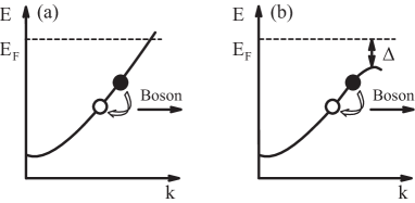
Figure 1: Bosonic scattering mechanism which contributes to the imaginary part of the self-energy. (a) normal state; (b) superconducting state.

In Fig. 2 (c) and (d) we have plotted the renormalization function Z(E) for the same parameters. The real part shows again a singularity at $\Omega_{0}$ and a constant value at zero energy. This value minus 1 again determines the coupling constant $\lambda^{b}_{n}$. Within this model the same coupling constant can also be obtained from the measurements of the quasiparticle linewidth at large negative energies as $\lambda^{b}_{n}=-2\Sigma^{{}^{\prime\prime}}(-\infty)/(\pi\Omega_{0})$. $\Sigma^{{}^{\prime\prime}}(-\infty)$ is the step height of $\Sigma^{{}^{\prime\prime}}(E)$ at $E$ = $\Omega_{0}$ in the one-mode model. Hence both $\lambda^{b}_{n}$ and $\Sigma^{{}^{\prime\prime}}(-\infty)$ are the measures of the coupling strength to the bosonic mode. Consequently, together with the mode energy $\Omega_{0}$, both can be used to determine the self-energy in the one-mode model.

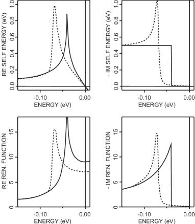
Figure 2: Real (a) and imaginary (b) part of the self-energy function and real (c) and imaginary (d) part of the renormalization function for a coupling to a mode at $\Omega_{0}$ = 40 meV and a coupling constant $\lambda_{n}$=8. Solid line: normal state, dashed line: superconducting state with a gap $\Delta$ = 30 meV

In Fig. 3 (a) and (b) we have displayed the calculated spectral function in the one-mode model for $\lambda^{b}_{n}=1$ and $\lambda^{b}_{n}=8$, respectively. Compared to the bare particle dispersion, $\epsilon_{k}$, given by the red dashed line, for |E| < $\Omega_{0}$ there is a mass renormalization, i.e., a reduced dispersion and no broadening, except the energy and momentum resolution broadening, which was taken to be 5 meV and 0.005 Å^-1, respectively . For |E| > $\Omega_{0}$, there is a dispersion back to the bare particle energy. Moreover, there is a broadening due to a finite $\Sigma^{\prime\prime}$, increasing with increasing $\lambda^{b}_{n}$. For large $\lambda^{b}_{n}$, the width for constant E scans is, at least up to some energy, larger than the binding energy of the charge carriers and therefore they can be called incoherent in contrast to energies |E| < $\Omega_{0}$ or very high binding energies, where the width is smaller than the binding energy and therefore the states are coherentSchrieffer . The change in the dispersion is often termed a "kink" but looking closer at the spectral function, in particular for high $\lambda^{b}_{n}$, there is a branching into two dispersion arms touching each other at the branching energy E_B=$\Omega_{0}$.

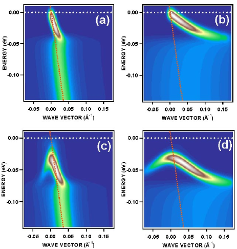
Figure 3: Calculated spectral function A(E,k) for a coupling of the charge carrier to a mode with an energy $\Omega_{0}$=40 meV (a) and (b) normal state, (c) and (d) superconducting state with a superconducting gap, $\Delta$=30 meV. (a) and (c) coupling constant $\lambda_{n}$=1, (b) and (d) coupling constant $\lambda_{n}$=8

The following information can be obtained from a one-mode model spectral function $A(E,k)$ in the normal state. When performing constant-E scans, very often called momentum distribution curves (MDCs), one obtains Lorentzians. The maximum observed in the MDCs determines the renormalized dispersion. By comparing this dispersion close to $E_{F}$ to the bare particle dispersion one can extract the coupling constant $\lambda^{b}_{n}$. The width of the Lorentzians for $|E|<\Omega_{0}$ in this model should be determined by the energy and momentum resolution. For $|E|>\Omega_{0}$ the resolution effects are small compared to the intrinsic width, W, and one can derive $\Sigma^{\prime\prime}(-\infty)=-v_{F}W/2$ where $v_{F}$ is the bare-particle Fermi velocity. From the onset of a finite intrinsic width, one obtains the mode energy $\Omega_{0}$. This parameter also can be obtained by constant-E cuts, very often called energy distribution curves (EDCs). Looking at Eq. (2), one realizes that for large $\epsilon_{k}$, i.e., far away from the Fermi wave vector, $k_{F}$, the spectral function around $E\sim\Omega_{0}$ is determined by $\Sigma^{\prime\prime}$. The edge of such a cut determines again $\Omega_{0}$.

In the superconducting state, the self-energy for $E<0$ is still given by (6), but the fermionic Green’s function now has the form

$$G_{sc}(E,k)=\frac{E+\epsilon_{k}}{E^{2}-\Delta^{2}-\epsilon^{2}_{k}+i\delta}$$ (9)

Substituting this into (6), evaluating the integral over $\epsilon_{k}$ and separating real and imaginary parts, we obtain for $E<0$:

$$\Sigma^{{}^{\prime}}(E)=-\frac{\lambda^{b}_{n}}{2}\Omega_{0}{\text{R}e}\int\frac{dE^{{}^{\prime}}}{\Omega^{2}_{0}-E^{{}^{\prime}2}-i\delta}\leavevmode\nobreak\ \frac{E+E^{{}^{\prime}}}{\sqrt{(E+E^{{}^{\prime}})^{2}-\Delta^{2}}}$$

$$\Sigma^{{}^{\prime\prime}}(E)=\frac{\pi}{2}\lambda^{b}_{n}\Omega_{0}{\text{R}e}\leavevmode\nobreak\ \frac{E+\Omega_{0}}{\sqrt{(E+\Omega_{0}+\Delta)(E+\Omega_{0}-\Delta)}}$$ (10)

In Fig. 2 we plot $\Sigma(E)$ and $Z(E)$ for the superconducting state with $\Delta$ = 30 meV. A small $\delta$ has been used to reduce the singularities. One realizes that due to the opening of the gap the singularities of $\Sigma^{\prime}$ and $Z^{\prime}$ are shifted to higher binding energies and that the edge in $\Sigma^{\prime\prime}$ transforms into an overshooting edge. At vanishing $E$, $\Sigma^{\prime}(E)$ is still linear in $E$, but due to the shift of the singularity to higher binding energies the slope is now reduced and given by

$$\lambda^{b}_{sc}=-\frac{\Sigma^{{}^{\prime}}(E\rightarrow 0)}{E}=\lambda^{b}_{n}\int_{0}^{\infty}\frac{dx}{(x^{2}+1)^{3/2}}\leavevmode\nobreak\ \frac{1}{1+x^{2}(\Delta/\Omega_{0})^{2}}$$ (11)

The reduction of the coupling constant in the superconducting state is concomitant with a reduction of $Z(0)$ since $Z(0)=1+\lambda$.

At $k=k_{F}$ the photohole can only be excited when its binding energy is exactly $\Delta$, or when $ImZ(E,k_{F})=-Im\Sigma(E,k_{F})/E$ is non-zero. From Fig. 1 (b) it is clear that for zero temperature and in the clean limit $\Sigma^{\prime\prime}$ or the scattering rate is different from zero only when $|E|>\Delta+\Omega_{0}$. This result is obtained from an evaluation of Eq. (10). This implies that $E=-\Delta$ is separated from the region where $\Sigma^{{}^{\prime\prime}}(E,k_{F})$ is non-zero and therefore the spectral function contains a $\delta-$functional peak at $E=-\Delta$, and then it becomes nonzero at $E<-(\Delta+\Omega_{0})$.

In Figs. 3 (c) and (d) we show for the one-mode model the calculated spectral function in the superconducting state using the same energy and momentum resolutions and the same mode energy as before. The gap was set to $\Delta$ = 30 meV. One clearly realizes the BCS-Bogoliubov-like back-dispersion at the gap energy $\Delta$ and besides this, a total shift of the dispersive arms by the gap energy. Thus the branching energy E_B occurs at $-(\Omega_{0}+\Delta)$.

The renormalized dispersion is obtained from the position of the MDC peak of the spectral function. In the normal state, the peak position is where the real part of $G^{-1}(E,k)$ vanishes. In the superconducting state, there is an extra complication due to the fact that $\epsilon_{k}$ is present both in the denominator and in the numerator of the spectral function. Like in an earlier study Chubukov we avoid this complication and extract the renormalized dispersion from

$$\epsilon_{k} = -{\text{R}e}Z(E)\sqrt{E^{2}-\Delta^{2}}$$ (12)

$$=-\left(1-\frac{{\text{R}e}\Sigma(E)}{E}\right)\sqrt{E^{2}-\Delta^{2}}.$$

In conventional superconductors, the mode energy is much larger than the gap. In this situation, Eq. (11) yields $\lambda^{b}_{sc}=\lambda^{b}_{n}\left(1+O\left((\Delta/\Omega_{0})^{2}\log{\Delta/\Omega_{0}}\right)\right)\approx\lambda^{b}_{n}$. Furthermore, the same small parameter $\Delta/\Omega_{0}$ also allows one to neglect the energy dependence of $\lambda_{sc,E}$ at $|E|\geq\Delta$, such that $\lambda^{b}_{sc,E}\approx\lambda^{b}_{sc}\approx\lambda^{b}_{n}$. In this situation, $ReZ(E)\approx 1+\lambda^{b}_{n}$, and hence the maximum of the spectral function is located at

$$E=-\sqrt{\Delta^{2}+\epsilon_{k}^{2}/(1+\lambda^{b}_{n})^{2}}.$$ (13)

For HTSCs, the gap is comparable to the mode energy and therefore Eq.(13) is no longer valid, and the full Eq. (12) should be used to fit the dispersion. There are two key differences with Eq. (13). First, the zero-energy values $\lambda^{b}_{sc}$ and $\lambda^{b}_{n}$ are different. For $\Delta=30$ meV and $\Omega_{0}=40$ meV, i.e., $\Delta/\Omega_{0}=3/4$, we obtain from (11) $\lambda^{b}_{sc}=0.74\lambda^{b}_{n}$. Second, the energy dependence of $\lambda^{b}_{sc}$ becomes relevant. Indeed, by analyzing (10) one finds that $\Sigma^{{}^{\prime}}(E)$ is discontinuous at $E=-(\Delta+\Omega_{0})$ and diverges as a square-root at approaching $E=-(\Delta+\Omega_{0})$. Chubukov When $\Delta$ and $\Omega_{0}$ are comparable, this divergence affects the self-energy already at $E\approx-\Delta$. For the parameters that we choose, the effect is not large: evaluating the real part of the self-energy at $E=-\Delta$ from (10) we find $\lambda^{b}_{sc,\Delta}\approx 1.1\lambda^{b}_{sc}$. However, the effect increases once $\Omega_{0}$ gets smaller.

Measuring an EDC at $k_{F}$ with high resolution, one would expect a peak at $\Delta$, followed by a region of near-zero spectral weight and a threshold of the incoherent spectral weight, which appears at $\Omega_{0}+\Delta$. Such an energy distribution is well known from tunnelling spectroscopy in conventional phonon superconductors, except that there $\Omega_{0}$ is often much larger than $\Delta$. At deviations from $k_{F}$, the peak disperses to larger frequencies while the onset of the incoherent spectral weight remains at $\Omega_{0}+\Delta$. Once the peak disperses close to $\Omega_{0}+\Delta$, only the threshold at this energy remains visible.

II.2 Collective mode model

For definiteness, we consider the model with the interaction between fermions and their spin collective excitations with momenta near $Q=(\pi,\pi)$. The momentum $Q$ connects Fermi surface points within antinodal regions, and hence antinodal fermions are mostly involved in the scattering of nearly antiferromagnetic spin fluctuations.

The physics of electron-boson interaction is somewhat different in the one-mode and collective mode scenarios. Like we said, in the one-mode formalism, one assumes that bosons are propagating excitations with a frequency $\Omega_{0}$, independent on whether fermions are in the normal or in the superconducting state. In the collective mode model, bosons are Landau-damped in the normal state, and their spectral function is described by a continuum rather than by a mode. In the superconducting state, the low-energy fermionic states in the antinodal regions are gapped, and the continuum of bosonic states with momenta near $Q$ appears only above the gap of $2\Delta$. In addition, the residual attraction between fermions in a $d_{x^{2}-y^{2}}$ superconductor leads to the development of the resonance peak at a frequency $\Omega_{0}$ below $2\Delta$. In the OD regime, $\Omega_{0}$ is only slightly below $2\Delta$, and the resonance is weak. In the UD regime, the resonance frequency decreases. In bilayer systems, such as Bi2212, there are two resonances, in the even and in odd channel. The resonance frequency in the even channel should vanish at the point where the magnetic correlation length diverges. The resonance in the odd channel remains finite at this point, and, very likely, transforms into the gapped spin-wave mode in the antiferromagnetically ordered state.

The self-energy within the collective mode model has been analyzed in Refr. Chubukov, and in earlier publications. Below we briefly review the existing results and also present several new formulas. For definiteness, we consider the case of a flat static susceptibility near $Q$, i.e., assume that in the normal state, the dynamical spin susceptibility (the bosonic propagator) can be expressed as

$$\chi(E,q)=\chi(E)=\frac{\chi_{Q}}{1-iE/\omega_{sf}}$$ (14)

where $\omega_{sf}$ is the typical relaxational frequency of spin fluctuations. An advantage of using the flat static spin susceptibility is that all computations can be done analytically. Similar results are also obtained using Ornstein-Zernike form of the static susceptibility Abanov and in FLEX computations for the Hubbard model manske .

In the normal state, the fermionic self-energy due to interaction with the gapless continuum of spin excitations is Chubukov

$$\Sigma^{{}^{\prime}}(E)=-\lambda^{c}_{n}\omega_{sf}\arctan{\frac{E}{\omega_{sf}}}$$

$$\Sigma^{{}^{\prime\prime}}(E)=-\frac{1}{2}\leavevmode\nobreak\ \lambda^{c}_{n}\omega_{sf}\ln(1+\frac{E^{2}}{\omega^{2}_{sf}})$$ (15)

where $\lambda^{c}_{n}$ is the dimensionless coupling constant in the normal state for the collective mode model. In distinction to the one-mode model, the self-energy in (15) has no threshold, and its energy dependence interpolates between different limits. In particular, $\Sigma^{{}^{\prime\prime}}(E)$ is quadratic in $E$ at the lowest energies (a Fermi-liquid form), and is almost flat at large $E$. At intermediate energies, $\Sigma^{{}^{\prime\prime}}(E)$ is roughly linear in $E$. The real part of the self-energy is linear in $E$ at the lowest frequencies ($-d\Sigma^{{}^{\prime}}(E)/dE_{E\rightarrow 0}=\lambda^{c}_{n}$), and is flat at high frequencies. If the relaxational spectrum of spin fluctuations is cut at some upper cutoff, the real part of the self-energy will start decreasing above the cutoff.

In the superconducting state, the self-energy changes by two reasons. First, fermionic excitations acquire a gap. Second, the spectrum of collective excitations by itself changes as a feedback from the gap opening. The expression for the self-energy incorporates both effects and is given by

$$\Sigma(E)=-\frac{1}{2}\lambda^{c}_{n}\leavevmode\nobreak\ \int\frac{dE^{{}^{\prime}}}{1-\Pi(E^{{}^{\prime}})/\omega_{sf}}\leavevmode\nobreak\ \leavevmode\nobreak\ \frac{E+E^{{}^{\prime}}}{\sqrt{(E+E^{{}^{\prime}})^{2}-\Delta^{2}}}$$ (16)

where $\Pi(E)$ is the polarizability bubble in the superconducting state (a sum of the two bubbles made of normal and anomalous fermionic Green’s functions). This polarization operator can be computed explicitly. We obtained

$$\Pi^{{}^{\prime}}(E)=\left\{\begin{array}[]{l}\frac{E^{2}}{2\Delta}D\left(\frac{E^{2}}{4\Delta^{2}}\right)\leavevmode\nobreak\ \mbox{for}\leavevmode\nobreak\ |E|<2\Delta\\ \\ \frac{4\Delta^{2}}{|E|}D\left(\frac{4\Delta^{2}}{E^{2}}\right)\leavevmode\nobreak\ \mbox{for}\leavevmode\nobreak\ |E|>2\Delta\end{array}\right.$$ (17)

$$\Pi^{{}^{\prime\prime}}(E)=\left\{\begin{array}[]{l}0\leavevmode\nobreak\ \mbox{for}\leavevmode\nobreak\ |E|<2\Delta\\ \\ |E|\leavevmode\nobreak\ K_{2}\left(1-\frac{4\Delta^{2}}{E^{2}}\right)\leavevmode\nobreak\ \mbox{for}\leavevmode\nobreak\ |E|>2\Delta\end{array}\right.$$ (18)

where $D(x^{2})=(K_{1}(x^{2})-K_{2}(x^{2}))/x^{2}$, and $K_{1}(x^{2})$ and $K_{2}(x^{2})$ are the elliptic integrals of first and second kind, respectively. The expression for $\Pi^{{}^{\prime\prime}}$ was earlier obtained in morr .

We see that $\Pi^{{}^{\prime\prime}}$ is finite only at $|E|>2\Delta$. At $|E|<2\Delta$, $\Pi^{{}^{\prime}}(E)$ is positive and interpolates between zero at $E=0$ and infinity at $|E|=2\Delta$ (at the lowest energies, $\Pi(E)\approx(\pi/8)E^{2}/\Delta$). At some frequency $\Omega_{0}$, $\Pi^{{}^{\prime}}(\Omega_{0})=\omega_{sf}$, and the dynamical spin susceptibility $\chi_{s}(E)\propto 1/(1-\Pi(E)/\omega_{sf})$ has a pole. As a result, the gapless continuum of the normal state splits into two separate entities: the gapped continuum at energies above $2\Delta$, where $\Pi^{{}^{\prime\prime}}$ is non-zero, and the pole (the resonance peak) at an energy $\Omega_{0}$ below $2\Delta$. We see therefore that in the superconducting state, one-mode and continuum models are quite similar – both describe the interaction between fermions and a bosonic mode. The difference between the two models is in the details, and also in the fact that in a collective mode model, the bosonic spectrum still contains a continuum above $2\Delta$.

The location of the pole can be straightforwardly obtained from (18). For $\Delta$ = 30 meV, the mode is at $\Omega_{0}$= 40 meV, if $\omega_{sf}\sim$ 26 meV. This last value is quite consistent with earlier estimates Abanov Near the pole, the spin susceptibility is

$$\chi(E)\approx Z_{0}\frac{\Omega_{0}}{\Omega^{2}_{0}-E^{2}-i\delta}$$ (19)

where $Z_{0}\sim 0.77$. Apart from the residue $Z_{0}$, Eq. (19) describes the same propagator as in the one-mode model (see Eq. (7)).

Substituting the results for $\Pi$ into the expression for the fermionic self-energy, Eq. (16), we find $\Sigma(E)$ as a sum of two contributions. One comes from the pole and the other comes from the gapped continuum. The generic behavior of the self-energy is similar to what we have found for the one-mode model. Namely, $\Sigma^{\prime}(E)$ is linear in $E$ at the lowest energies, and diverges as a square-root at approaching $-(\Delta+\Omega_{0})$ from below. Above this threshold, $\Sigma^{{}^{\prime}}(E)$ drops to a finite value, and decreases at even larger $|E|$. The imaginary part of the self-energy is zero below the threshold at $-(\Delta+\Omega_{0})$, diverges as a square-root at approaching the threshold from larger $|E|$, and eventually recovers the normal state value at highest energies. At the smallest $E$, we found that the dominant contribution to $\Sigma^{\prime}(E)=-\lambda^{c}_{sc}E$ comes from the mode, continuum only accounts for about 20% percent correction. Evaluating the integrals, we found that $\lambda^{c}_{sc}\approx 0.7\lambda^{c}_{n}$. This is similar to what we have found in the one-mode model. At $E=-\Delta$, we found, using the full form of the polarization bubble, $\lambda^{c}_{sc,\Delta}\approx 0.75\lambda^{c}_{n}$, which is again similar to what we have found in the one-mode model.

For the imaginary part of the self-energy $\Sigma^{{}^{\prime\prime}}(E)$ and $E$ < 0 we found

$$\Sigma^{{}^{\prime\prime}}(E)=\Sigma^{{}^{\prime\prime}}_{A}(E)+\Sigma^{{}^{\prime\prime}}_{B}(E)$$ (20)

where

$$\Sigma^{{}^{\prime\prime}}_{A}(E)=\frac{\pi Z_{0}}{2}\lambda^{c}_{n}\Omega_{0}\frac{E+\Omega_{0}}{(E+\Omega_{0}+\Delta)(E+\Omega_{0}-\Delta)}$$

$$\Sigma^{{}^{\prime\prime}}_{B}(E)=-\lambda^{c}_{n}\int_{2\Delta}^{|E|}dx\text{Re}\frac{E+x}{\sqrt{(E+x)^{2}-\Delta^{2}}}\leavevmode\nobreak\ \times$$

$$\frac{\frac{x}{\omega_{sf}}K_{2}(1-\frac{4\Delta^{2}}{x^{2}})}{\left(1-\frac{4\Delta^{2}}{x\omega_{sf}}D(\frac{4\Delta^{2}}{x^{2}})\right)^{2}+\left(\frac{x}{\omega_{sf}}K_{2}(1-\frac{4\Delta^{2}}{x^{2}})\right)^{2}}$$ (21)

The first contribution is from the mode, the second is from the gapped continuum. At $-(\Omega_{0}+\Delta)>E>-3\Delta$ only the mode contributes. The self-energy in this range is very similar to the one-mode result. Above $3\Delta$, the gapped continuum also contributes to $\Sigma^{{}^{\prime\prime}}(E)$, initially as $\sqrt{E+3\Delta}/\log^{2}(E+3\Delta)$ for $E\leq-3\Delta$, and more strongly at larger $|E|$. Combining the contributions from the mode and from the gapped continuum, we found numerically that the total $\Sigma^{{}^{\prime\prime}}$ is almost flat above $3\Delta$ at a value $\Sigma^{{}^{\prime\prime}}\approx 1.5\lambda^{c}_{n}\Omega_{0}$. The near-constant value of $\Sigma^{{}^{\prime\prime}}$ is quite close to the normal state value in the one-mode model, $\Sigma^{{}^{\prime\prime}}_{n}=(\pi/2)\lambda^{b}_{n}\Omega_{0}$, but we stress that in the collective mode model, this flat behavior is obtained at $|E|\approx 3\div 5\Delta$. In the one-mode model, $\Sigma^{{}^{\prime\prime}}(E)$ at these energies has a strong frequency dependence ranging between $1.25\Sigma^{{}^{\prime\prime}}_{n}$ at $E=-3\Delta$ to $1.04\Sigma^{{}^{\prime\prime}}_{n}$ at $E=-5\Delta$.

II.3 Comparison and application of the two models

Not surprisingly, one-mode and collective mode models give very different results for the normal state. Within the one-mode model, the normal state spectral function still shows a peak-dip-hump structure, and the renormalized dispersion displays an $S$-shape structure near $E=-\Omega_{0}$. In the collective mode model, the imaginary part of the self-energy is roughly linear in $E$ at frequencies comparable to $\Omega_{0}$, and $\Sigma^{{}^{\prime}}(E)$ displays a crossover from a linear behavior at small frequencies to a near constant behavior at higher frequencies. From this perspective, a combination of the measurements below and above $T_{c}$ provides the best way to distinguish between the two models, particularly as we found the relation between the coupling constants in the normal and superconducting states. Several ARPES measurements near $(\pi,0)$ indicate Kim ; Gromko ; Sato that the coupling to the mode disappears above T_c thus strongly supporting the collective mode model.

The normal state measurements may be “contaminated” by thermal effects, which mask the difference between the two models. A way to avoid thermal effects is to focus on low $T$ measurements. However the two models give very similar results for the superconducting state. The only qualitative difference is the gapped continuum which is still present in the collective mode model, but the continuum affects the self-energy only in a moderate extent both at vanishing $E$ and at $|E|\sim\Delta$. The dominant contribution to the self-energy at these energies comes from the resonance at $\Omega_{0}$, which is present in both models. The continuum does affect the self-energy at $|E|\sim 3\div 5\Delta$, but it is difficult to measure the self-energy in the $(\pi,0)$ region in this energy range since the bare dispersion only extends to $\sim 2\Delta$ for the antibonding band and to $\sim 7\Delta$ for the bonding band and therefore all evaluations strongly depend on the exact values of the bare particle dispersion.

On the other hand, the close similarity between the two models in the superconducting state is good for addressing the fundamental issue whether the data in the superconducting state are actually consistent with the collective mode model, and with estimates of $\lambda^{c}_{sc}$ or $\lambda^{c}_{n}$.

For the analysis of the experimental data we used the one-mode model which is determined by $\lambda^{b}_{sc}$ and which simulates the coupling to the magnetic resonance mode. neutron The bare one-mode model is extended by adding to the self-energy a Fermi-liquid-like term which is shifted by 3$\Delta$ to higher binding energy. This term approximates the gapped continuum and is determined by the coupling constant $\lambda^{f}_{sc}$. We then compare the two coupling constants $\lambda^{b}_{sc}$ and $\lambda^{f}_{sc}$ with theoretical estimates for the coupling constant $\lambda^{c}_{sc}$ in the collective mode model. Abanov ; Abanov3 We obtain reasonable agreement between experiment and theory which indicates that the dressing of the charge carriers in the ($\pi$,0) region is related to a coupling of spin excitations. We also show that the magnitude $\Sigma^{\prime\prime}(-\infty)$ evaluated from the incoherent spectral weight is consistent with the value of $\lambda^{b}_{n}$ derived from the dispersion near $\Delta$. This means that the spectral function for the coherent and the incoherent states can be described by one self-energy function indicating a common linear dressing for the both states.

III Experimental setup

The ARPES experiments were carried out at the BESSY synchrotron radiation facility using the U125/1-PGM beam line and a SCIENTA SES100 analyser. Spectra were taken with various photon energies ranging from 17 to 65 eV. The total energy resolution ranged from 8 meV (FWHM) at photon energies h$\nu$=17-25 eV to 22.5 meV at h$\nu$=65 eV. The momentum resolution was set to 0.01 Å^-1 parallel to the $(\pi,0)-(\pi,\pi)$ direction and 0.02 Å^-1 parallel to the $\Gamma-(\pi,0)$ direction. Here we focus on spectra taken with photon energies of 38 eV and 50 (or 55 eV) to discriminate between bonding and antibonding bands. The polarization of the radiation was along the $\Gamma-(\pi,0)$ direction. Measurements have been performed on (1$\times$5) superstructure-free, optimally doped BiPb2212 single crystal with a T_c= 89 K. Since data for the normal state have already been published Kim we only show data measured at T = 30 K.

IV Experimental Results

In Fig. 4 we show typical ARPES data for wave vectors close to the $(\pi,\pi)-(\pi,-\pi)$ line, centered around the $(\pi,0)$ point.

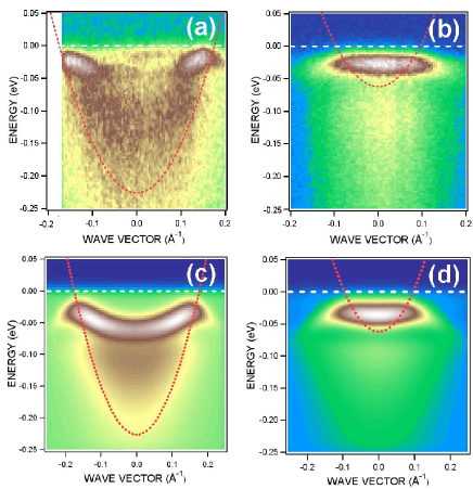
Figure 4: ARPES intensity plots as a function of energy and wave vectors along the $(\pi,\pi)-(\pi,-\pi)$ direction of the optimally doped Pb-Bi2212 superconductor taken at T = 30 K. Zero corresponds to the $(\pi,0)$ point. (a) bonding band, (b) antibonding band. (c) and (d): calculated spectral function using a model self-energy function for the region around the $(\pi,0)$ point. The red dashed line represents the bare-particle bandstructure

As has been shown previouslyBorisenko3 ; Kordyuk5 ; Kim and supported by theoretical calculationsBansil ; Fujimori , the data taken with h$\upsilon$=38eV due to matrix element effects represent mainly the bonding band with some contributions from the antibonding band. The data taken at h$\upsilon$=50 eV (see Fig. 4(b)) have almost pure antibonding character. In order to obtain the spectral weight of the pure bonding band (see Fig. 4(a)), a fraction of the 50 eV data has been subtracted from the 38 eV data. We have also added in Fig. 4 the bare-particle dispersion which was obtained from a self-consistent evaluation of the data at the nodal pointKordyuk3 , an evaluation of the anisotropic plasmon dispersionNucker ; Grigoryan and from LDA bandstructure calculationsAndersen . When comparing this bare-particle dispersion with the very broad distribution of the bonding band at high energies, one realizes a renormalization of the occupied bandwidth by a factor of about 1.7 corresponding to $\lambda^{f}_{sc}\approx 0.7$. This value is not far from that derived for the bandwidth renormalization above T_c, where no additional renormalization effects at lower energies have been detected, Kim and from that at the nodal point Kordyuk3 ; Kordyuk5 . Probably a large fraction of this bandwidth renormalization stems from a coupling of the charge carriers to the above mentioned continuum of spin fluctuationsAbanov .

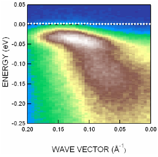
Figure 5: ARPES intensity plot for k-values near the $(1.4\pi,\pi)-(1.4\pi,-\pi)$ line of the optimally doped Pb-Bi2212 superconductor taken at T = 30 K. Zero corresponds to the $(1.4\pi,0)$ point. The data were taken with a photon energy h$\upsilon$ = 50 eV in order to maximize the intensity of the antibonding band.

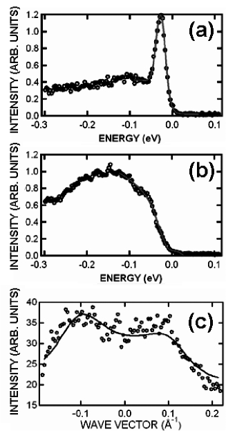
Figure 6: (a) Constant-k cut of the data shown in Fig 5 at k_F; (b) constant-k cut of the data at about one third of k_F (starting at the $(\pi,0)$ point); (c) constant-E cut at E = -100 meV. The solid lines represent fits to the data (see text)

In Fig. 5 we show an ARPES intensity distribution near k_F of the antibonding band, close to the $(1.4\pi,\pi)-(1.4\pi,-\pi)$ line, of Pb-Bi2212 measured at 30 K with a photon energy h$\upsilon$ = 50 eV. At this place in the second Brillouin zone, the bare particle dispersion of the antibonding band reaches well below $E_{B}$ = 70 meV and therefore contrary to Fig. 4 (b) the branching into two dispersive arms can be clearly realized. These data together with the data of Fig. 4 when compared with the model calculations shown in Fig. 3 clearly reveal that the dominant effect of the renormalization, besides the bandwidth renormalization mentioned above, is due to a coupling to a bosonic mode leading to a branching energy of $\sim$ 70 meV.

In order to obtain more quantitative information on the parameters which determine the self-energy function leading to this renormalization we have performed various cuts of the spectral weight shown in Fig. 4 (a) which are presented in Fig. 6. A constant-k scan for k=k_F is depicted in Fig. 6(a) showing the typical peak-dip-hump structure presented for data taken at the $(\pi,0)$ point in previous studies Norman ; Borisenko3 . From the peak energy one can derive the superconducting gap energy $\Delta$ = 30(4) meV. In the previous literatureEschrig , from the dip energy at $\sim$ 70 meV the branching energy E_B was derived. Another constant-k scan at 1/3 k_F (starting from the $(\pi,0)$ point) is shown in Fig. 6(b). At this k-value the intensity of the coherent peak is strongly reduced and in the framework of the one-mode model, mainly the threshold of the incoherent states (the hump) is observed. From a fit to these data, taking into account a small intensity of the coherent line and a threshold of the incoherent states, the threshold energy could be determined which in the one-band model yields the branching energy, $E_{B}=\Delta+\Omega_{0}$ = 70(5)( meV. This together with the gap energy $\Delta$= 30 meV yields a mode energy of 40 meV.

In Fig. 6(c) we show a constant-energy cut at $E$ = -100 meV of the data presented in Fig. 4. As discussed in Sect. II, from the fit of those cuts with a Lorentzian one can obtain from the width of the Lorentzian a value of the imaginary part of the self-energy at the selected energy. For the energy below the mode energy, this value $\Sigma^{\prime\prime}(-\infty)$ is a measure of the coupling to the mode. The actual situation is more complicated since near the antinodal point, the bandstructure is far from being linear at this energy range. We have fitted the data shown in Fig. 6(c) by Eq. (4) with the self-energy given by (8), the bare dispersion extracted from earlier work, Kim $\Delta$ = 30 meV, $\Omega_{0}$ = 40 meV, and $\Sigma^{\prime\prime}(-\infty)$ used as a parameter. Moreover as described above a Fermi-liquid like term was added to the self-energy to approximate the influence of the gapped continuum. The imaginary part of this term is given by $\alpha(E-3\Delta)^{2}$ for $|E|>3\Delta$ and zero for $|E|<3\Delta$ where the magnitude of $\alpha$ is determined by $\lambda^{f}_{sc}$. The value $3\Delta$ can be easily understood by looking at Fig. 1 since in the superconducting state the states available for a fermion decay have minimum energy of $3\Delta$, and hence below $3\Delta$, the correction to $\Sigma^{{}^{\prime\prime}}$ from the continuum is zero. Using this self-energy function from an extended one-mode model the fit yielded typical values for the parameter $\Sigma^{\prime\prime}(-\infty)$ as shown in Fig. 7. For $|E|>E_{B}$ = 70 meV the values should be constant. The finite slope detected in the analysis may be related to errors in the bare particle dispersion, to the assumption of a constant density of states during the definition of the self-energy function, or to in the assumed $\lambda^{f}_{sc}$. For $|E|<E_{B}$ the results from the fits are determined by the flat dispersion of the coherent states and therefore, due to the finite energy resolution, large values are obtained in this energy range (not shown). From evaluations of such data taken on several samples we derive a value $\Sigma^{\prime\prime}(-\infty)$ = 130(30) meV. The large error for this value stems from various measurements on samples with slight mismatches in there orientation which leads to different bare bandstructures as compared to the assumed one.

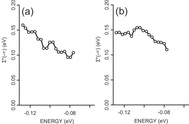
Figure 7: Typical values for $\Sigma^{\prime\prime}(-\infty)$ as derived from a fit of constant-E cuts (see Fig. 6) of data shown in Fig. 4(a) and (b) using Eq. (4) The solid line is a guide to the eyes. (a) bonding band, (b) antibonding band.

Another important information comes from the dispersion of the coherent spectral weight between the gap energy $-\Delta$ and the branching energy $-(\Delta+\Omega_{0})$. Originally Kim ; Gromko , the data were fitted using Eq. (13). As pointed out in Sect. II this is a good approximation for conventional superconductors, where the mode energy is much higher than the gap, but not for the high-T_c superconductors. Here the energy of the mode is comparable to the gap energy and therefore the renormalization function from which the $\lambda^{b}_{sc}$ -values are derived, depends on energy and also on $\Delta/\Omega_{0}$. In this communication we have fitted the data using the full Eqs. (4) and (12). For the complex self-energy function, we have used the same parameters as for the fit of the constant-energy cuts shown in Fig. 6 (c). We then obtain a complex renormalization function Z(E) from which we derive $\lambda$-values not at energies between $\Delta$ and $\Delta+\Omega$ as in the previous studyKim but at zero energy, i.e., $\lambda^{b}_{sc}=Z(0)-1$. In the fit we have used the above given values for $\Delta$ and $\Omega_{0}$ and we have chosen $\lambda^{b}_{sc}$ as a parameter. From the fit, we extracted $\lambda_{sc}^{b}=2.0(4)$. This yields a total $\lambda_{sc}^{t}$= 2.7(5) from Z(0) in the superconducting state composed of a bandwidth renormalization part $\lambda_{sc}^{f}=0.7(3)$ and a bosonic part $\lambda_{sc}^{b}=2.0(4)$. The errors are not due to statistics but result from different measurements on different samples. Using the relation $\lambda^{b}_{sc}=0.74\lambda^{b}_{n}$ (see Sec.  II) we obtain $\lambda^{b}_{n}=2.7$. To obtain $\lambda^{f}$ in the normal state we used the same $Im\Sigma$ from fermion-fermion interaction as in the superconducting state, but set $\Delta$ = 0. This yields $\lambda^{f}_{n}\sim 1.3$ and a total coupling constant for the normal state $\lambda_{n}^{t}=4.0(5)$. We collected the values of the coupling constants and $\Sigma^{\prime\prime}(-\infty)$ in Table II. Note that the normal state values are not derived from measurements in the normal state. Rather they were derived from data taken in the superconducting state and setting $\Delta$ to zero in the renormalization function. This means that $\lambda^{b}_{n}$ in Table II is a fictitious normal state coupling constant because the bosonic mode does not exist in the normal state. It is only presented for the comparison of the coupling constant in HTSCs with those of conventional metals and superconductors.

Table 2: Parameters determining the self-energy function of Pb-Bi2212 near $((\pi,0)$ below T_c. $\lambda^{f}$, $\lambda^{b}$, $\lambda^{t}$, coupling constants from bandwidth renormalization, from coupling to a bosonic mode, and total coupling constant, respectively. $\Sigma^{\prime\prime}(-\infty)$ is determining the imaginary part of the self-energy function at high binding energies. sc: parameters derived in the superconducting state, n: parameters calculated for the normal state by setting $\Delta$ to zero. The data are compared with parameter derived for a Mo(110) surface state Valla and for Pb Reinert

system	$\lambda^{f}$	$\lambda^{b}$	$\lambda^{t}$	$\Sigma^{\prime\prime}(-\infty)(meV)$
BiPb2212 sc	0.7(3)	2.0(4)	2.7(5)	130(30)
BiPb2212 n	1.3(3)	2.7(4)	-	130(30)
Mo(110)	-	0.4	-	15
Pb n	-	1.6	-	-

V Discussion

The coupling constant to a bosonic mode was derived from the dispersion of the coherent states between -30 and -70 meV while $\Sigma^{\prime\prime}(-\infty)$ was derived from a constant-E cut of the incoherent states below -70 meV. If the data can be described by one self-energy function which essentially results from a coupling to one bosonic mode, the $\lambda^{b}_{n}$-value calculated from $\Sigma^{\prime\prime}(-\infty)$ within this model should agree with the $\lambda_{n}^{b}$-value extracted from the dispersion of the coherent states. Using the relation $\lambda_{n}^{b}=-2\Sigma^{\prime\prime}(-\infty)/(\pi\Omega_{0})$ (see Sect. II) and the value $\Sigma^{\prime\prime}(-\infty)$ = 130(30) meV one obtains $\lambda_{n}^{b}$ = 2.1(5) which is in reasonable agreement with $\lambda_{n}^{b}\sim 2.7(4)$ derived from the dispersion near $-\Delta$. This supports the idea that the coherent and the incoherent spectral weight of the spectral function in the superconducting state can be described by a single self-energy function, which is essentially determined by the coupling to one bosonic mode at 40 meV. This view is also supported by the fact that taking this self-energy function and calculating the spectral function using Eq. (2) we obtain a reasonable agreement with the experimental ARPES data, both for the bonding and the antibonding band (see Fig. 4). The differences in the intensities of the bonding band near ($\pi$,0) may be explained by matrix element effects. We emphasize that in the superconducting state both the real and the imaginary part of the self-energy function indicate a very strong coupling to a bosonic mode.

Recently, there has been some evidence from ARPES measurements KShen ; Roesch that in the undoped cuprates there is a very large electron-phonon coupling leading to a strong polaronic renormalization connected with a negligible spectral weight for the coherent states and a high spectral weight for a multiphononic line at higher energies. Furthermore there are theories of the pairing in high-T_c superconductors which are based on the formation of polarons and bipolaronsAlexandrov . The big question is whether this strong electron-phonon coupling survives for the high-T_c superconductors or whether it will be screened by the charge carriers and at what dopant concentration the adiabatic approximation is valid, where the Fermi energy is much larger than the mode energy. The data shown in Fig. 5, which were actually taken down to an energy of -400 meV, show no indication of a polaronic line at lower energy. Moreover, the data in Fig. 5 and its evaluation in terms of a coupling to a single bosonic mode gives no room for multi-bosonic polaron excitations for optimally doped samples.

The analysis given above clearly identifies below T_c a very strong coupling to a bosonic mode. In Table II we have listed other coupling constants to bosonic (phonon) modes detected by ARPES. Compared to the surface state of the Mo(110) surface coupled to a phonon mode, $\lambda_{n}^{b}$ in OPBiPb2212 is a factor of 6 larger. Almost the same factor 8 is obtained for $\Sigma^{\prime\prime}(-\infty)$. Compared to the strong coupling superconductor Pb the coupling constant $\lambda_{n}^{b}$ for OP BiPb2212 is a factor of 1.6 larger. This indicates that we really have a very strong coupling to a bosonic mode. This coupling is even enhanced at lower dopant concentration Kim .

In the following we compare the experimental coupling constants $\lambda^{f}_{sc}$ and $\lambda^{b}_{sc}$ with those derived in the collective mode model for the gapped continuum and for the single mode, respectively. In the collective mode model, in the superconducting state about 20 % of the total coupling constant comes from the gapped continuum (see Sec. II B). The corresponding experimental value $\lambda^{f}_{sc}/\lambda^{t}_{sc}$ = 0.26 (see Table II) is in remarkable agreement with the theoretical value. This also holds for the absolute values of the coupling constant. In previous work Abanov ; Abanov3 the normal state coupling constant for the collective mode model was estimated to be $\lambda^{c}_{n}=2\div 3$ from fits of theoretical values for $\omega_{sf}$, $\Omega_{0}$, and $T_{c}$. This transforms into $\lambda^{c}_{sc}=1.5\div 2.25$ for the superconducting state which is not far from the experimental value $\lambda^{t}_{sc}$ = 2.7(5). Thus the agreement of the relative and absolute experimental values of the coupling constants with those derived from the collective mode model is a strong indication that the dressing of the charge carriers in the ($\pi$,0) region (i.e. the region were the superconducting order parameter has its maximum) is predominantly determined by a coupling to spin excitations, in particular to the magnetic resonance mode.

This interpretation is supported by several other ARPES results. The strong temperature dependence of the coupling to the mode Kim ; Gromko is difficult to understand in terms of electron phonon coupling. Our model calculations also show that the data above T_c cannot be described by a thermally broadened phonon line. Also the strong dopant dependence Kim ; Gromko is difficult to be explained in terms of electron phonon coupling. Furthermore there is a large coupling at $(\pi,0)$ and a much smaller coupling to the mode at the nodal point, indicating a coupling of states which are separated by a wavevector $(\pi,\pi)$ typical of an antiferromagnetic susceptibility. Moreover the energy of the bosonic mode detected in ARPES is close to the energy of the magnetic resonance mode detected in inelastic neutron scattering. Finally we mention recent ARPES measurements on the parity of the coupling between bonding and antibonding band BorisenkoP and the ”magnetic isotope effect”, i.e., the strong changes of the dressing of the charge carriers upon substitution of Cu by Zn. Ding ; Zabolo , which both support the magnetic scenario.

VI Conclusion

In this contribution we have analyzed the spectral function of optimally doped BiPb2212 near the antinodal points measured by ARPES. Compared to previous studies, we have not analyzed just one constant-k cut or just the dispersion of the coherent state but the entire spectral function including the coherent and the incoherent spectral weight. In this context we have used expressions which not only can be used in the case of normal superconductors but also for HTSCs where the mode energy is not much larger than the superconducting gap. It was possible to describe the spectral function using a single parameterized self-energy function. By comparison of the experimental data with theoretical models, we conclude that the main contribution to the self-energy is a very strong coupling to the magnetic resonance mode. At higher energies (and above T_c) it was necessary to take into account a bandwidth renormalization by a factor of two due to interaction with a gapped (ungapped) continuum of spin excitations.There is no evidence for multi-bosonic polaron excitations for this dopant concentration.

Acknowledgments

We thank S.V. Borisenko and A.A. Kordyuk for helpful discussions. Financial support by the DFG Forschergruppe under Grant No. FOR 538 is acknowledged. One of the authors (J.F.) appreciates the hospitality during his stay at the Ames Laboratories. A. Chubukov is supported by NSF-DMR 0240238.

References

- (1) A. Damascelli, Z.-X. Shen, and Z. Hussain, Rev. Mod. Phys. 75, 473 (2003)
- (2) J.C. Campuzano, M.R. Norman, and M. Randeria, Photoemission in the High-Tc Superconductors. In: Physics of Superconductors, vol II, ed by K.H. Bennemann and J.B. Ketterson (Springer, Berlin Heidelberg New York 2004) pp 167-273
- (3) Jörg Fink, Sergey Borisenko, Alexander Kordyuk, Andreas Koitzsch, Jochen Geck, Volodymyr Zabalotnyy, Martin Knupfer, Bernd Büchner, and Helmut Berger cond-mat/0512307.
- (4) D.S. Dessau, B.O. Wells, Z.-X. Shen, W.E. Spicer, A.J. Arko, R.S. List, D.B. Mitzi, and A. Kapitulnik, Phys. Rev. Lett. 66,2160(1991).
- (5) M.R. Norman, H. Ding, J.C. Campuzano, T. Takeuchi, M Randeria, T. Yokoya, T. Takahashi, T. Mochiku, and K. Kadowaki, Phys. Rev. Lett. 79,3506(1997).
- (6) A. Kaminski, M. Randeria, J.C. Campuzano, M.R. Norman, H. Fretwell, J. Mesot, T. Sato, T. Takahashi, and K. Kadowaki, Phys. Rev. Lett. 86, 1070 (2001)
- (7) T. Sato, H. Matsui, T. Takahashi, H. Ding, H.-B. Yang, S.-C. Wang, T. Fujii, T. Watanabe, A. Matsuda, T. Terashima, and K. Kadowaki, Phys. Rev. Lett. 91, 157003 (2003)
- (8) T.K. Kim, A.A. Kordyuk, S.V. Borisenko, A. Koitzsch, M. Knupfer, H. Berger, and J. Fink, Phys. Rev. Lett. 91, 167002 (2003)
- (9) A.D. Gromko, A. V. Fedorov, Y.D. Chuang, J.D. Koralek, Y Aiura, Y. Yamaguchi, K. Oka, Yoichi Ando, and D.S. Dessau, Phys. Rev. B 68, 174520 (2003).
- (10) Ar. Abanov and A.V. Chubukov, Phys. Rev. Lett. 83, 1652 (1999).
- (11) W. L. McMillan and J. M. Rowell, Tunneling and Strong Coupling Superconductivity, in Superconductivity, Vol. 1, p. 561, Ed. Parks, Marull, Dekker Inc. N.Y. (1969).
- (12) A.A. Kordyuk, S.V. Borisenko, T.K. Kim, K.A. Nenkov, M. Knupfer, J. Fink, M.S. Golden, H. Berger,and R. Follath, Phys. Rev. Lett. 89, 077003 (2002)
- (13) S.V. Borisenko, A.A. Kordyuk, T.K. Kim, A. Koitzsch, M. Knupfer, M.S. Golden, J. Fink, M. Eschrig, H. Berger, and R. Follath, Phys. Rev. Lett. 90, 207001 (2003)
- (14) A. Bansil and M. Lindroos, Phys. Rev. Lett. 83, 5154 (1999)
- (15) J.D. Lee and A. Fujimori, Phys. Rev. Lett. 87, 167008 (2001)
- (16) A. A. Kordyuk, S. V. Borisenko, M.S. Golden, S. Legner, K.A. Nenkov, M. Knupfer, J. Fink, H. Berger, L. Forro, and R. Follath, Phys. Rev. B 66, 014502 (2002)
- (17) A.A. Kordyuk, S.V. Borisenko, M. Knupfer, and J. Fink, Phys. Rev. B 67, 064504 (2003)
- (18) A.A. Kordyuk, S.V. Borisenko, V. B. Zabolotnyy, J. Geck, M. Knupfer, J. Fink, B. Büchner, C. T. Lin, B. Keimer, H. Berger, Seiki Komiya, and Yoichi Ando, cond-mat/0510760
- (19) A.V. Chubukov and M.R. Norman, Phys. Rev. B 70, 174505 (2004).
- (20) M.R. Norman and H. Ding, Phys. Rev. B 57, R11089 (1998)
- (21) K.M. Shen, F. Ronning, D.H. Lu, W.S. Lee, N.J.C. Ingle, W. Meevasana, F. Baumberger, A. Damascelli, N.P. Armitage, L.L. Miller, Y. Kohsaka, M. Azuma, M. Takano, H. Takagi, and Z.-X. Shen, Phys. Rev. Lett. 93, 267002 (2004).
- (22) O. Rösch and O. Gunnarsson: Phys. Rev. Lett. 92, 146403 (2004).
- (23) S. Engelsberg and J. R. Schrieffer, Phys. Rev. 131, 993 (1963)
- (24) D. J. Scalapino, in Superconductivity, vol. 1, ed. R. D. Parks (Marcel Decker, New York 1969), p. 449.
- (25) M. Eschrig and M. R. Norman, Phys. Rev. Lett. 85, 3261 (2000) and Phys. Rev. B 67 144503 (2003); M. Eschrig, cond-mat 0510286.
- (26) T.P. Devereaux, T. Cuk, Z.-X. Shen, and N. Nagaosa, Phys. Rev. Lett. 93, 117004 (2004).
- (27) G.D. Mahan, Many-Particle Physics, (Plenum Press, New York 1990)
- (28) L. Hedin and S. Lundquist, Solid State Physics 23, 1963 (1969)
- (29) C.O. Almbladh and L. Hedin, Beyond the one-electron model in Handbook of Synchrotron Radiation, vol 1b, ed by E.E. Koch (North Holland, Amsterdam 1983) pp 607-904.
- (30) Y. Nambu, Phys. Rev. 117, 648 (1960).
- (31) A. Abanov, A. V. Chubukov, J.Schmalian, Journal of Electron Spectroscopy and Related Phenomena 117, 129 (2001); A. Abanov, A.V. Chubukov, and J. Schmalian, Adv. Phys. 52, 119 (2003); Ar. Abanov, A. Chubukov, and A. Finkelstein, Europhys. Lett. 54, 488 (1999).
- (32) C. Timm, D. Manske, and K. H. Bennemann, Phys. Rev. B 66, 094515 (2002); T. A. Maier, M. S. Jarrell, and D. J. Scalapino, Phys. Rev. Lett. 96, 047005 (2006).
- (33) H. Westfahl and D.K. Morr, Phys. Rev. B 62, 5891 (2000).
- (34) J. Rossat-Mignod, L.P. Regnault, C. Vettier, P. Bourges, P. Burlet, J. Bossy, J.Y. Henry, G. Lapertot, Physica C 185-189, 86 (1991); H. A. Mook, M. Yethiraj, G. Aeppli, T.E. Mason, T. Armstrong: Phys. Rev. Lett. 70, 3490 (1993); H. F. Fong, B. Keimer, P.W. Anderson, D. Reznik, F. Dogan, I.A. Aksay: ibid. 75, 316 (1995).
- (35) A. Abanov, A.V. Chubukov, M. Eschrig, M.R. Norman, and J. Schmalian, Phys. Rev. Lett. 89, 177002 (2002).
- (36) N. Nücker, U. Eckern, J. Fink, and P. Müller, Phys. Rev. B 44, 7155 (1991)
- (37) V.G. Grigoryan, G. Paasch, and S.-L. Drechsler, Phys. Rev. B 60, 1340 (1999)
- (38) O.K. Andersen, A.I. Liechtenstein, O. Jepsen, and F. Paulsen, J. Phys. Chem. Solids 56, 1573 (1995)
- (39) A.A. Kordyuk, S.V. Borisenko, A. Koitzsch, J. Fink, M. Knupfer, and H. Berger, Phys. Rev. B 71, 214513 (2005)
- (40) T. Valla, A.V. Fedorov, P.D. Johnson, and S.L. Hulbert, Phys. Rev. Lett. 83, 2085 (1999)
- (41) F. Reinert, B. Eltner, G. Nicolay, D. Ehm, S. Schmidt, and S. Hüfner, Phys. Rev. Lett. 91, 186406 (2003)
- (42) A.S. Alexandrov, The Theory of Superconductivity: From Weak to Strong Coupling (IoP Publishing, Bristol and Philadelphia, 2003)
- (43) S.V. Borisenko, A.A. Kordyuk, A. Koitzsch, J. Fink, J. Geck, V. Zabolotnyy, M. Knupfer, B. Büchner, H. Berger, M. Falub, M.Shi, J. Krempasky, and L. Patthey, Phys. Rev. Lett. 96, 067001 (2006)
- (44) K. Terashima, H. Matsui, D. Hashimoto, T. Sato, T. Takahashi, H.Ding, T. Yamamoto, and K. Kadowaki, Nature Physics 2, 27(2006).
- (45) V.B. Zabolotnyy, S.V. Borisenko, A.A. Kordyuk, J. Fink, J. Geck, A. Koitzsch, M. Knupfer, B. Büchner, H. Berger, A. Erb, C.T. Lin, B. Keimer, R. Follath, Phys. Rev. Lett. 96,037003 (2006)