Phase behaviour and particle-size cutoff effects in polydisperse fluids

Abstract

We report a joint simulation and theoretical study of the liquid-vapor phase behaviour of a fluid in which polydispersity in the particle size couples to the strength of the interparticle interactions. Attention is focussed on the case in which the particles diameters are distributed according to a fixed Schulz form with degree of polydispersity $\delta=14\%$. The coexistence properties of this model are studied using grand canonical ensemble Monte Carlo simulations and moment free energy calculations. We obtain the cloud and shadow curves as well as the daughter phase density distributions and fractional volumes along selected isothermal dilution lines. In contrast to the case of size-independent interaction strengths (N.B. Wilding, M. Fasolo and P. Sollich, J. Chem. Phys. 121, 6887 (2004)), the cloud and shadow curves are found to be well separated, with the critical point lying significantly below the cloud curve maximum. For densities below the critical value, we observe that the phase behaviour is highly sensitive to the choice of upper cutoff on the particle size distribution. We elucidate the origins of this effect in terms of extremely pronounced fractionation effects and discuss the likely appearance of new phases in the limit of very large values of the cutoff.

PACS numbers: 64.70Fx, 68.35.Rh

I Introduction and background

When the constituent particles of a many body system exhibit variation in terms of some attribute such as their size, shape or charge, then that system is termed “polydisperse”. Occurring, as it does, in soft matter systems as diverse as colloids, polymers and liquid crystals, the phenomenon of polydispersity is both widespread and basic. However, owing to the complexity that polydispersity bestows on a system, gaining an understanding of its physical consequences represents a considerable challenge to theory, simulation and experiment alike. Meeting this challenge is not solely a matter of fundamental concern, but also one of practical importance: the presence of polydispersity in substances of commercial and industrial importance (such as paints, fuels and foodstuffs) is known to profoundly affect their thermodynamic and processing properties in ways which are as yet neither well characterized nor well understood LARSON99 ; FREDRICKSON ; RUSSEL89 .

Of the many fundamental questions that polydispersity elicits, one of the most central concerns its influence on bulk phase separation. The phase behavior of polydisperse fluids is known to be considerably richer in both variety and character than that of their monodisperse counterparts GUALTIERI82 ; SOLLICH02 . This richness has its source in fractionation effects EVANS98 ; EVANS01 ; HEUKELUM03 ; SHRESTH02 ; EDELMAN03 ; FAIRHURST04 ; ERNE05 ; WILDING04 : the distribution of the polydisperse attribute differs from one coexisting phase to another. In order to quantify this effect, it is expedient SALACUSE to regard the polydisperse attribute as a continuous variable $\sigma$, and to define a density distribution $\rho(\sigma)$, where $\rho(\sigma)d\sigma$ is the number density of particles in the range $\sigma\ldots\sigma+d\sigma$. Fractionation then occurs when, at two phase coexistence, a “parent” density distribution $\rho^{(0)}(\sigma)$ splits into two distinct “daughter” phase distributions $\rho^{(1)}(\sigma)$ and $\rho^{(2)}(\sigma)$. Particle conservation implies that the daughter distributions are related to the parent via a simple volumetric average:

$$(1-\xi)\rho^{(1)}(\sigma)+\xi\rho^{(2)}(\sigma)=\rho^{(0)}(\sigma)\>,$$ (1)

where $1-\xi$ and $\xi$ are the fractional volumes of the two phases.

Experimentally, the situation typically considered (for example in studies of colloidal dispersions) is the nature of the phase behaviour along a so-called dilution line. Here, one takes a sample of some prescribed polydispersity and observes its coexistence properties as it is progressively diluted by adding solvent, the temperature being held constant. Under such circumstances the parent distribution maintains a fixed shape, and only its overall scale varies according to the degree of dilution. Accordingly, one can write

$$\rho^{(0)}(\sigma)=n^{(0)}f^{(0)}(\sigma)\>,$$ (2)

where $f^{(0)}(\sigma)$ is a fixed shape function which serves to define the form of the polydispersity, while $n^{(0)}$ is the overall (parent) number density of the system, whose value parameterizes the location of the system on the dilution line.

In order to construct the full phase diagram for such a system one must obtain the dilution line phase behaviour for the range of temperatures of interest. However, in contrast to a monodisperse system where the limits of phase stability and the densities of the coexisting phases are completely specified by the coexistence binodal in the $n^{(0)}-T$ plane, fractionation implies that polydispersity splits the binodal into cloud and shadow curves SOLLICH02 , as shown schematically in fig. 1. These curves mark, respectively, the density of the onset of phase separation and the density of the incipient (shadow) daughter phase. For parent densities lying wholly within the coexistence region, two daughter phases form, the properties of which vary non-trivially with $n^{(0)}$. Hence a full specification of the coexistence properties of a polydisperse system requires not only a determination of the locus of the cloud curve, but also the dependence of $\xi$, $\rho^{(1)}(\sigma)$ and $\rho^{(2)}(\sigma)$ on $n^{(0)}$ and $T$.

Figure 1: A schematic fluid-fluid phase diagram for a polydisperse fluid, showing temperature $T$ against density; the cloud curve gives the parent density $n^{(0)}$ where phase separation first occurs while the shadow curve records the density of the incipient coexisting phases. Note, however, that the shadow phase density distribution lies off the dilution line.

In the present work, we describe a joint simulation and theoretical study of liquid-vapor phase separation for a model fluid in which polydispersity affects not only the length scale but also the strength of the interaction potential. Previously we have considered the restricted case of size-independent interaction strengths, for which the critical point is found to lie very close to the maximum of the cloud curve WILDING04 . By contrast, for the present model it is located substantially below the maximum (cf. fig. 1), as is observed in many experiments on complex fluids (see e.g. DOBASHI ). One implication of this is that phase coexistence occurs at and above the critical temperature, provided the overall parent density is less than its critical value, and we investigate this feature here. Another difference to the case of size-independent interactions is an acute sensitivity of the coexistence properties to the presence of rare large particles. We study this phenomenon by varying a particle size cutoff parameter.

As regards previous simulation studies of polydisperse phase equilibria, other authors have (to date) considered exclusively the case of variable polydispersity, in which the shape of the parent distribution changes according to the temperature and overall density STAPLETON ; BOLHUIS ; KOFKE93 ; KRISTOF ; PRONK04 ; BATES98 . As such, these studies do not reflect the most commonly encountered experimental situation in which the polydispersity of a system is fixed by the process of its chemical synthesis. With the recent advent of bespoke Monte Carlo (MC) simulation techniques WILDING03 ; WILDING04 , however, studies of fixed polydispersity within the (appropriate) grand or semi-grand canonical ensemble framework are now tractable. In the present work we apply these methods to study the phase separation of a fluid whose polydispersity assumes a prescribed functional form.

A number of analytical studies of polydisperse phase equilibria have also been reported in the literature. These typically seek to calculate the system free energy as a function of a set of density variables. Unfortunately, this task is complicated by the fact that the requisite free energy $f[\rho^{(0)}(\sigma)]$ is a functional of $\rho^{(0)}(\sigma)$, and therefore occupies an infinite dimensional space. For sufficiently simple model free energies which generalize the van der Waals (vdW) approximation, a direct attack on the solution of the phase equilibrium conditions is nevertheless sometimes possible, see e.g. GUALTIERI82 ; XU00 . The reason for this is that such models are normally “truncatable” SOLLICH01 so that the phase equilibrium conditions can be reduced to nonlinear equations for a finite number of variables. This approach has been applied to the study of phase separation in fluids exhibiting separate size and interaction strength polydispersity, yielding predictions for the cloud and shadow curves and critical parameters as a function of polydispersity BELLIER00 . An alternative approach which more systematically exploits the advantages of truncatable models is the moment free energy (MFE) method SOLLICH01 ; SOLLICH02 . This approximates the full free energy appropriately in terms of a “moment free energy” which depends on a small number of density variables, thereby permitting the efficient use of standard tangent plane construction to locate phase boundaries. The MFE method delivers (for the given model free energy) exact results for the location of critical points and the cloud and shadow curves. With appropriate refinements, it can also be used to obtain exact numerical solutions to the phase coexistence conditions when two or more phases coexist in finite amounts ClaCueSeaSolSpe00 ; SOLLICH01 ; SpeSol02 ; SpeSol03a . The MFE method has been applied to the study of phase behaviour in systems ranging from polydisperse hard rods to the freezing of hard spheres SOLLICH02 ; FASOLO03 ; KALY03 ; KALY04 ; RASCON03 , and we shall deploy it again here to study the phase behaviour of the present model, based on a refined van der Waals-type approximation to the excess free energy.

Our paper is organized as follows PRL . In sec. II we introduce our model, a polydisperse Lennard-Jones (LJ) fluid that we study via grand canonical Monte Carlo (MC) simulation and the MFE method. Additionally we sketch the MC simulation methodology and provide some brief background to the MFE calculations. Sec. III details our estimates for the cloud and shadow curves, as well as the behaviour of the fractional volumes of the daughter phases and their density distributions along selected isothermal dilution lines in a range including the critical temperature. We then turn in sec. IV to a consideration of the effects of the choice of the upper cutoff on the particle size distribution. Our results demonstrate that coexistence properties can be acutely sensitive to this choice. We elucidate the origin of this sensitivity in terms of the interplay between the rate of decay of the parent size distribution at large $\sigma$, and the $\sigma$-dependence of the excess chemical potential. Likely implications for the phase behaviour at very large cutoffs are also discussed. Finally, Sec. V details out conclusions and highlights some outstanding questions worthy of further investigation.

II Model and methodologies

II.1 Simulation model

We consider a polydisperse Lennard-Jones fluid whose interparticle potential takes the form:

$$u_{ij}=\epsilon_{ij}\left[\left({\sigma_{ij}}/{r_{ij}}\right)^{12}-\left({\sigma_{ij}}/{r_{ij}}\right)^{6}\right]$$ (3)

with interaction strength $\epsilon_{ij}=\sigma_{i}\sigma_{j}$ and interaction radius $\sigma_{ij}=(\sigma_{i}+\sigma_{j})/2$; $r_{ij}=|{\bf r}_{i}-{\bf r}_{j}|$ denotes the separation between the particles. A truncation was applied to the potential for $r_{ij}>2.5\sigma_{ij}$ and no tail corrections were used.

With regard to the form of this potential, a couple of remarks are appropriate. Firstly, although it differs from that studied in Ref. WILDING04 only in the $\sigma$-dependence of the interaction strength parameter $\epsilon_{ij}$, we shall show that this difference is crucial in determining many of the qualitative aspects of the phase behavior of the model. Secondly, the form of Eq. (3) might, in one sense, be regarded as somewhat artificial because for vanishingly small particles the interaction strength approaches zero. An arguably more realistic form would be a repulsive hard core plus an attractive well of variable strength. However, it transpires that for the form of parent distribution studied in the present work this drawback is of minor significance since the physics of the system is dominated by the largest particles.

II.2 Parent distribution

Throughout this work we consider the case in which the particle diameters $\sigma$ are drawn from a (parental) distribution of the Schulz form SCHULZ :

$$f^{(0)}(\sigma)=\frac{1}{z!}\left(\frac{z+1}{\bar{\sigma}}\right)^{z+1}\sigma^{z}\exp\left[-\left(\frac{z+1}{\bar{\sigma}}\right)\sigma\right]\>,$$ (4)

with a mean diameter $\bar{\sigma}$ which sets our unit length scale. We have elected to study the case $z=50$, corresponding to a moderate degree of polydispersity: the standard deviation of particle sizes is $\delta\equiv 1/\sqrt{z+1}\approx 14\%$ of the mean. The form of the distribution is shown in Fig. 2. Although our motivation for employing the Schulz distribution is primarily ad-hoc, we note that it has been found to fairly accurately describe the polydispersity of some polymeric systems MCDONNEL .

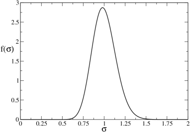
Figure 2: Schulz distribution for the case $z=50$ (cf. Eq. (4)).

In both the simulations and the MFE calculations described below, the distribution $f^{(0)}(\sigma)$ was limited to within the range $0.5<\sigma<\sigma_{c}$. The upper cutoff $\sigma_{c}$ serves to prevent the appearance of arbitrarily large particles in the simulation, but would also be expected in experiment because in the chemical synthesis of colloid particles, time or solute limits restrict the maximum particle size KVITEK05 . Various choices of $\sigma_{c}$ have been considered, and these are discussed in relation to the results of Secs. III and IV.

II.3 Simulation strategy

The phase behaviour of the polydisperse LJ model Eq. 3) was studied via MC simulations within the grand canonical ensemble (GCE). The MC algorithm invokes four types of operation: particle displacements, deletions, insertions, and resizing. The particle diameter $\sigma$ is treated as a continuous variable in the range $0\leq\sigma\leq\sigma_{c}$, with $\sigma_{c}$ the prescribed cutoff. However, distributions defined on $\sigma$ such as the instantaneous density $\rho(\sigma)$, and the chemical potential $\mu(\sigma)$, are represented as histograms defined by discretising the permitted range of $\sigma$ into $120$ bins. Most of the simulation results presented below pertain to a periodic cubic system of linear dimension $L=15\bar{\sigma}$, although near the critical point, where finite-size effects are important, we determined the phase behaviour using system sizes ranging up to $L=30\bar{\sigma}$. For further details concerning the simulation algorithm, as well as the structure, storage and acquisition of data, we refer the interested reader to ref. WILDING02 .

The principal observable of interest is the fluctuating form of the instantaneous density distribution $\rho(\sigma)$. From this we derive the distribution $p(n)$ of the overall number density $n=\int d\sigma\rho(\sigma)$, and that of the volume fraction $\eta=(\pi/6)\int d\sigma\sigma^{3}\rho(\sigma)$. The existence of phase coexistence at given chemical potentials is signalled by the presence of two distinct peaks in the probability distribution $p(n)$. In order to obtain estimates of dilution line coexistence properties at some prescribed temperature, we employ an approach recently proposed by ourselves in Ref. BUZZACCHI06 . For a given choice of $n^{(0)}$, the method entails tuning the chemical potential distribution $\mu(\sigma)$ together with a parameter $\xi$, such as to simultaneously satisfy both a generalized lever rule and an equal peak weight criterion BORGS for $p(n)$:

$$n^{(0)}f^{(0)}(\sigma) = (1-\xi)\rho^{(1)}(\sigma)+\xi\rho^{(2)}(\sigma)$$ (5a)

$$r = 1$$ (5b)

Here the daughter density distributions $\rho^{(1)}(\sigma)$ and $\rho^{(2)}(\sigma)$ are assigned by averaging only over configurations belonging to either peak of $p(n)$. The quantity $r$ is the peak weight ratio:

$$r=\frac{\int_{n>n^{*}}p(n)dn}{\int_{n<n^{*}}p(n)dn}\>,$$ (6)

with $n^{*}$ a convenient threshold density intermediate between vapor and liquid densities, which we take to be the location of the minimum in $p(n)$. The tuning of $\mu(\sigma)$ and $\xi$ necessary to simultaneously satisfy Eqs. (5a) and (5b) can be efficiently achieved by a combination of histogram extrapolation techniques HR , and a non-equilibrium potential refinement (NEPR) procedure as described elsewhere WILDING03 .

The value of $\xi$ resulting from the application of the above procedure is the desired fractional volume of the liquid phase at the nominated value of $n^{(0)}$. Cloud points are determined as the value of $n^{(0)}$ at which $\xi$ first reaches zero (vapor branch) or unity (liquid branch), while shadow points are given by the density of the coexisting incipient daughter phase, which may be simply read off from the appropriate peak density in the cloud point form of $p(n)$. It should be pointed out that the finite-size corrections to estimates of coexistence properties obtained using the equal peak weight criterion for $p(n)$ are exponentially small in the system size BUZZACCHI06 .

In order to obtain the phase behaviour of our model system, we scanned the dilution line for a selection of fixed temperatures. We started by setting $T=T_{c}$, the critical temperature, and tracked the locus of the dilution line in a stepwise fashion. This tracking procedure must be bootstrapped with knowledge of the form of $\mu(\sigma)$ at some initial point on the dilution line. A suitable estimate was obtained, for a point near the critical density, by means of the NEPR procedure WILDING03 , in conjunction with the equal peak weight criterion for $p(n)$, discussed above. Simulation data accumulated at this near-critical state point was then extrapolated to a lower, but nearby density $n^{(0)}$ by means of histogram reweighting, thus providing an estimate of the corresponding form of $\mu(\sigma)$. The latter was employed in a new simulation, the results of which were similarly extrapolated to a still lower value of $n^{(0)}$. Iterating this procedure thus enabled the systematic tracking of the whole dilution line. Histogram extrapolation further permitted a determination of dilution line properties at adjacent temperatures, thereby facilitating a systematic determination of the phase behaviour in the $n^{(0)}-T$ plane. Implementation of multicanonical preweighting techniques BERG92 at each coexistence state point ensured adequate sampling of the coexisting phases in cases where they are separated by a large interfacial free energy barrier (see refs. WILDING04 ; WILDING01 for a fuller account of this latter procedure).

II.4 Moment free energy method

We complement the simulations with theoretical phase behaviour calculations, following closely our study of the purely size-polydisperse case WILDING04 . To find a suitable expression for the excess free energy density $f^{\rm ex}$, we approximate the repulsive part of our LJ interaction as completely hard. The resulting contribution to $f^{\rm ex}$ is represented accurately by the BMCSL approximation $f^{\rm ex}_{\rm BMCSL}$ BOUBLIK ; MANSOORI ; SALACUSE :

$$\frac{\pi}{6}\beta f^{\rm ex}_{\rm BMCSL}=\left(\frac{\rho_{2}^{3}}{\rho_{3}^{2}}-\rho_{0}\right)\ln(1-\rho_{3})+\frac{3\rho_{1}\rho_{2}}{1-\rho_{3}}+\frac{\rho_{2}^{3}}{\rho_{3}(1-\rho_{3})^{2}}\;.$$

This is a function of the moments up to third order of the density distribution, $\rho_{i}=(\pi/6)\int\!d\sigma\,\sigma^{i}\rho(\sigma)$ ($i=0,\ldots,3$); note that $\rho_{0}=(\pi/6)n$ is proportional to the overall number density, while $\rho_{3}=\eta$ is the volume fraction. We have set $k_{\rm B}=1$ and defined $\beta=1/T$ as usual so that $\beta f^{\rm ex}$ has dimension of density.

We treat the remaining attractive part of the LJ interaction potential in the simplest possible way, by adding a quadratic van der Waals term to the excess free energy. Using the fact that the interaction volume of two particles of diameters $\sigma$ and $\sigma^{\prime}$ scales as $(\sigma+\sigma^{\prime})^{3}$, while the interaction strength $\epsilon_{ij}$ is proportional to $\sigma\sigma^{\prime}$, this can be written as

$$\frac{\pi}{6}\beta f^{\rm ex}_{\rm vdW} = -\frac{1}{2t}\left(\frac{\pi}{6}\right)^{2}\int\!d\sigma\,d\sigma^{\prime}\,\rho(\sigma)\rho(\sigma^{\prime})(\sigma\sigma^{\prime})(\sigma+\sigma^{\prime})^{3}$$ (7)

$$= -\frac{1}{t}(\rho_{1}\rho_{4}+3\rho_{2}\rho_{3})$$

where $t$ is an appropriate dimensionless temperature. Given the approximate character of the overall excess free energy $f^{\rm ex}=f^{\rm ex}_{\rm BMCSL}+f^{\rm ex}_{\rm vdW}$, it would not make sense to try to scale $t$ precisely to the temperature in the simulations. Instead, we will be content to study whether our $f^{\rm ex}$ can reproduce the qualitative trends observed in the simulations. While still somewhat crude, it should be better suited to this task than previous versions BELLIER00 because it incorporates polydispersity not only into the attractive contribution, but also into the hard core reference system.

As pointed out in the introduction, to predict phase equilibria for polydisperse systems is generally still a computationally demanding task even if an explicit expression for the excess free energy is available SOLLICH02 . The above excess free energy has the simplifying feature that it only depends on the finite set of moments $\rho_{0},\ldots,\rho_{4}$, i.e. it is truncatable SOLLICH01 . This allows us to exploit the MFE method to obtain accurate numerical predictions for the phase behaviour. We refer the interested reader to our analogous study of the purely size-polydisperse case for a fuller description of the methodology WILDING04 .

III Phase behaviour: general aspects

We have employed the simulation and MFE methods outlined in the previous section to determine the cloud and shadow curves for our system. Various choices of the particle size cutoff have been considered, although the majority of our simulation results pertain to the cases $\sigma_{c}=1.4$ and $\sigma_{c}=1.6$. Referring to Fig. 2 it is clear that both values are quite far out into the tail of the parent size distribution, and naively one would therefore expect only very minor differences. Our results, expressed in the $n$-$T$ representation, are shown in Fig. 3(a) (for simulations of the LJ model) and Fig. 3(b) (for MFE predictions). In both cases we observe a strong separation of cloud and shadow curves; as a consequence the critical point lies well below the cloud curve maximum. We also note a pronounced difference in the cloud curves for the two cutoffs, contrary to naive expectation; detailed discussion of this effect is deferred to Sec. IV.

Finite-size scaling methods WILDING95 (specifically the matching of $p(n)$ to its known universal critical point form) were utilized to provide accurate estimates of the critical parameters of the LJ model. These yielded $n^{(0)}_{c}=0.326(3)$, $T_{c}=1.375(2)$ (for $\sigma_{c}=1.4$); $n^{(0)}_{c}=0.329(3)$, $T_{c}=1.384(2)$ (for $\sigma_{c}=1.6$), which are to be compared with those of the monodisperse LJ fluid WILDING95 : $n^{(0)}_{c}=0.3196(4)$, $T_{c}=1.1876(3)$. Thus polydispersity of the form considered here acts to raise the critical temperature substantially, although the associated increase in the critical density is much more modest. We note that a polydispersity-induced increase in $T_{c}$ has also been observed for the case of size-independent interaction strengths WILDING04 . There, however, the magnitude of the shift in $T_{c}$ was only around $5\%$ of that seen in the present model, for the same parent distribution.

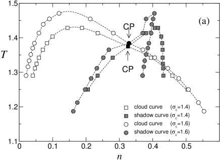
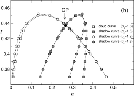
Figure 3: Cloud and shadow curves in the $n-T$ plane. (a) MC simulation results. (b) MFE predictions. Lines are a guide to the eye.

The MFE results of Fig. 3(b) show qualitatively very similar behaviour to the simulation results: the high density part of the shadow curve has an unusual positive slope which becomes more pronounced as the cutoff increases; at the same time the maxima of cloud and shadow curves shift to higher temperatures. Quantitatively the cutoff effects are somewhat weaker than in the simulations, which is why we chose to display results for $\sigma_{c}=1.6$ and 1.9 rather than 1.4 and 1.6 as for the simulations.

One difference between simulations and theory is the nature of the cloud and shadow curves in the vicinity of the critical point. In the simulation results “dips” are observable in this region, in contrast to the MFE results which show no such effect. The precise origin of the dips is not clear to us at present. One possibility is that they are a finite-size effect caused by the breakdown near the critical point of our procedure for determining cloud points. Alternatively they may be indicative of genuine critical point singularities in the cloud and shadow curves which are not picked up by the theory because our approximate free energy expression is of a mean-field type.

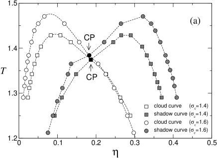
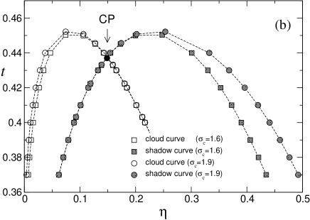
Figure 4: Cloud and shadow curves in the $\eta-T$ plane. (a) MC results. (b) MFE predictions. Lines are a guide to the eye.

In Fig. 4 we show the forms of the cloud and shadow curves in the $\eta$-$T$ representation, i.e. plotting on the $x$-axis the volume fraction $\eta$ rather than the density $n$ of the cloud and shadow phases. Since the cloud phase always has the fixed parental size distribution, the cloud curve is simply rescaled by this change of representation; the same is not true of the shadow curve, however, since the size distribution in the shadow varies throughout the phase diagram. As a consequence, we observe that in the volume fraction plot the cloud and shadow curves separate even further than before, forming a rather symmetrical “butterfly” shape. Again there is good qualitative agreement with the MFE predictions.

Turning now to the coexistence properties inside the coexistence region, we plot, in Figs. 5 and 6, the measured $n^{(0)}$ dependence of the number densities and volume fractions of the coexisting vapor and liquid phases on the critical isotherm. In the MC simulations, these were obtained simply by reading off the peak positions of $p(n)$ and $p(\eta)$ for the appropriate values of $n^{(0)}$ and $T$. Close to the critical point, one expects large finite-size effects to occur due to the divergent correlation length. These are indeed apparent in our measurements of the peak densities of $p(n)$ and $p(\eta)$ for a number of system sizes (see insets of Figs. 5(a) and 6(a)). Specifically, since the form of $p(n)$ is doubly peaked for finite-sized systems, even at the critical point WILDING95 , one expects that the peak densities approach the critical density as a universal power law in the system size, $L^{-\beta/\nu}$. This convergence to the critical density is indeed visible in the insets of Figs. 5(a) and 6(a), although we have not attempted to verify the anticipated scaling behaviour explicitly.

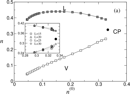
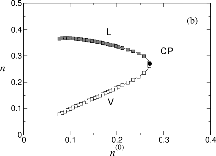
Figure 5: (a) MC results for the number densities of the coexisting vapor and liquid phases as a function of $n^{(0)}$ at $T=T_{c}$, for $\sigma_{c}=1.6$. The inset expands the near-critical region and shows data for a number of system sizes (expressed in units of $\bar{\sigma}$), as indicated. (b) MFE predictions.

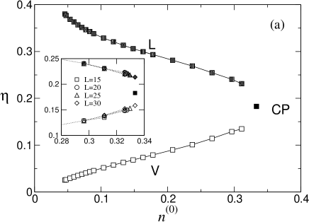
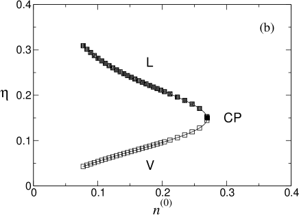
Figure 6: (a) MC results for the volume fraction of the coexisting vapor and liquid phases as a function of $n^{(0)}$ at $T=T_{c}$, for $\sigma_{c}=1.6$. The inset expands the near-critical region and shows data for a number of system sizes. (b) MFE predictions.

With regard to the behavior of the coexistence number densities as a function of parent density $n^{(0)}$ away from criticality (Fig. 5), we find that the liquid phase density varies non-monotonically, while the vapor density decreases as the gas phase branch of the cloud curve is approached. These trends are also seen in the corresponding MFE results, though the non-monotonicity in the liquid density is much weaker and only just perceptible on the scale of the figure. In the volume fraction representation (Fig. 6), on the other hand, the liquid volume fraction increases monotonically as the gas cloud curve is approached, while the vapor volume fraction decreases. Thus the effect of isothermally reducing $n^{(0)}$ from its critical value is analogous to that seen on lowering the temperature isochorically in a monodisperse system: the difference in the volume fraction of the two coexisting phases increases.

This aspect of the phase behaviour is also manifest in the $n^{(0)}$ dependence of the surface tension, which may be estimated from the form of $p(n)$ via BINDER82

$$\gamma=\lim_{L\to\infty}\frac{1}{2L^{d-1}}\ln\left[\frac{p^{\rm max}(n)}{p^{\rm min}(n)}\right]$$ (8)

where $p^{\rm max}(n)/p^{\rm min}(n)$ is the ratio of the peak to trough probabilities of the order parameter distribution, which provides a measure of the free energy cost of a planar interface. Formally Eq. (8) is valid only in the limit of sufficiently large system sizes, where the pair of liquid-vapor interfaces (whose presence is mandated by the periodic boundary conditions) are effectively non-interacting. Although we have been unable to study systems sufficiently large to fully approach this limit in the vicinity of the critical point, we do regard our results for $\gamma$ as representative of the bulk for parent densities $n^{(0)}<0.29$. Fig. 7 shows our estimates of the surface tension for three isotherms having temperatures $T<T_{c}$, $T=T_{c}$ and $T>T_{c}$. One sees that in each instance the surface tension starts at a large finite value on the gas branch of the cloud curve, but rapidly decreases with increasing parent density. On approaching the high density cloud point it falls to zero for $T=T_{c}$ as expected for critical phase coexistence, while for $T>T_{c}$ and $T<T_{c}$ it decreases to a finite value as is more clearly visible in the inset of Fig. 7.

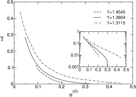
Figure 7: Surface tension $\gamma$ for three isotherms at $T>T_{c}$, $T=T_{c}$ and $T<T_{c}$ and size cutoff $\sigma_{c}=1.6$; the inset shows the same data on a logarithmic scale to emphasize the behaviour near the respective liquid (high density) cloud points.

Finally in this section, we point out qualitative differences in the nature of the coexistence behaviour above and below the critical temperature. Fig. 8 plots our simulation estimates of $\xi$, the fractional volume of the liquid [cf. Eq. (1)], as a function of $n^{(0)}$ for the same three isotherms as considered above. For the case $T<T_{c}$, the fractional volume of the liquid is zero at the gas phase cloud, and steadily increases with $n^{(0)}$ – in a non-linear fashion – to reach $\xi=1$ at the liquid phase cloud point. By contrast for $T=T_{c}$, $\xi$ increases from zero at the gas phase cloud, but reaches a maximum of $\xi=0.5$ at the critical point. Finally for $T>T_{c}$, $\xi$ starts from zero, increases to a maximum, and then decreases to zero again as the high density branch of the cloud curve is reached. Thus the distinguishing feature of the “supercritical” (in temperature, i.e. $T\geq T_{c}$) coexistence region is that the fractional volume of the liquid phase never reaches unity. The corresponding MFE predictions show the same qualitative behaviour (data not shown).

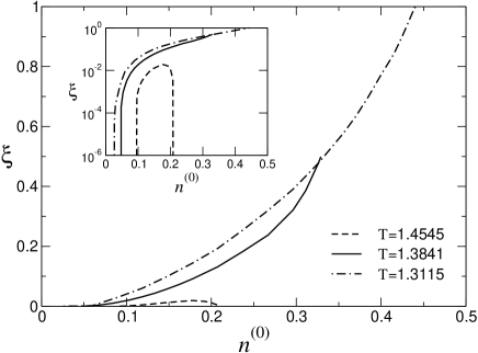
Figure 8: MC results for the fractional volume of the liquid phase $\xi$ as a function of parent density $n^{(0)}$ across the coexistence region, for three isotherms $T>T_{c}$, $T=T_{c}$ and $T<T_{c}$ and size cutoff $\sigma_{c}=1.6$. Inset: Same data on a logarithmic scale.

IV Phase behaviour: cutoff effects

We return now to address the striking feature evident from Figs. 3 and 4 of a large difference in the measured cloud and shadow curves for the two cutoffs $\sigma_{c}=1.4$ and $1.6$. Specifically, the gas phase cloud curve for $\sigma_{c}=1.6$ is shifted to much lower densities compared to that for $\sigma_{c}=1.4$. This occurs even though both values of $\sigma_{c}$ are far in the tail of the parent distribution [cf. Fig. 2]. The origin of this effect is to be found in the character of the particle size distributions in the liquid daughter phase. Fig. 9 shows the form of this distribution for selected values of $n^{(0)}$ on the critical isotherm for $\sigma_{c}=1.6$. One observes that as the gas cloud point density is approached from above, there is a progressive accumulation of weight in the large-$\sigma$ region of the distribution. Thus despite the fact that particle sizes around $\sigma_{c}$ are very rare in the parent, they occur (by virtue of fractionation) in much higher concentrations in the liquid. The physical basis for this is the stronger interaction between the larger particles [cf. Eq. (3)]; an enhancement in the concentration of such particles then yields a substantial free energy gain at the shorter interparticle separations of the liquid.

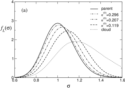
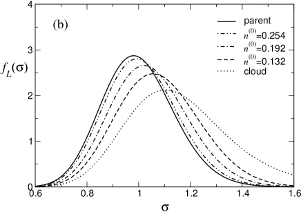
Figure 9: Liquid phase size distributions $f_{L}(\sigma)$ for a selection of values of $n^{(0)}$ spanning the coexistence region at $T=T_{c}$. Data are shown for cutoff $\sigma_{c}=1.6$. (a) MC results. (b) MFE predictions; densities were chosen to be at the same relative positions across the coexistence region as for (a).

Clearly, therefore, the choice of cutoff has a profound effect on the liquid daughter phase distribution, particularly in the low density region close to the cloud point where the fractionation-induced enhancement of the large-$\sigma$ tail of the size distribution in the liquid is greatest. The magnitude of the truncation effect at the gas phase cloud point, for $T=T_{c}$, is quantified in Fig. 10(a), which compares the measured forms of the shadow phase size distribution at cutoffs $\sigma_{c}=1.4,\sigma_{c}=1.6$ and $\sigma_{c}=1.8$. For these cutoff values, we find that the density at $\sigma=\sigma_{c}$ is enhanced compared to the corresponding parent density by factors of $11.9(1)$, $175(7)$ and $5280(50)$ respectively. Also shown, in Fig. 10(b), are the corresponding MFE results for the same choice of cutoffs, together with a further distribution for the larger cutoff $\sigma_{c}=3$; we discuss the form of the latter below.

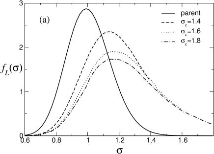
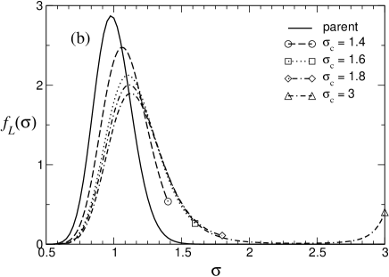
Figure 10: (a) Size distributions $f_{L}(\sigma)$ in the liquid shadow phase at $T=T_{c}$ for $\sigma_{c}=1.4,1.6,1.8$, together with the parent distribution $f^{(0)}(\sigma)$ plotted for comparison. (b) MFE predictions, including the larger cutoff $\sigma_{c}=3$.

Given that the liquid shadow phase distribution is highly sensitive to the cutoff and that this phase coexists with the gas cloud phase, the origin of the sensitivity of the locus of the cloud curve to the choice of cutoff [as seen in Figs. 3 and 4] becomes clear. We can now also rationalize the observation that such significant cutoff effects are restricted to parent densities below the critical density. For higher densities, the shadow phase is a gas of lower density than the parent. In this, the concentration of large particles is suppressed and that of small particles negligibly enhanced because of their weak interactions. The shadow size distributions are therefore concentrated well within the range $0.5\ldots\sigma_{c}$ so that no noticeable cutoff dependence arises.

The observed decrease in the gas cloud point density $n_{\rm cl}^{(0)}$ with increasing $\sigma_{c}$ prompts the question as to whether the gas phase cloud point density would eventually tend to a zero or nonzero limit as $\sigma_{c}$ is increased. Fig. 11 shows the simulation results and MFE predictions on the critical isotherm. The former exhibit a further strong decrease of $n^{(0)}_{\rm cl}$ by $\approx 25\%$ between $\sigma_{c}=1.6$ and $1.8$; the latter suggest that this trend continues and that the cloud point density tends to zero for large $\sigma_{c}$. Such an unusual effect has previously been seen in theoretical studies of polydisperse hard rods with broad length distributions SpeSol03a and in a Flory-Huggins model for polymers SOLC . It is also predicted to occur in solid-solid phase separation of polydisperse hard spheres HS_longpaper , though only for large $\sigma_{c}$ and distributions with fatter than exponential tails. In the present model, however, the decrease of $n^{(0)}_{\rm cl}$ is clear even for $\sigma_{c}$ of $O(1)$, i.e. of the same order as $\bar{\sigma}$. The physical origin of the decrease of $n^{(0)}_{\rm cl}$ to zero is the appearance (for large $\sigma_{c}$) of a second peak in the shadow phase size distribution near $\sigma_{c}$ (Fig. 10(b)). As with hard rods, we expect this second peak to eventually dominate as $\sigma_{c}$ increases so that the shadow phase comprises ever more strongly interacting particles whose sizes are concentrated near $\sigma_{c}$. The appearance of the second peak in the size distribution also correlates directly with a significant extension of the coexistence region towards smaller parent densities, as shown in Fig. 12. This extension shifts the cloud point to lower densities, leaving in its wake a region where the fractional volume occupied by the liquid phase is extremely small, below $10^{-6}$. This region then crosses over at parent densities around $n^{(0)}=0.06$ to more conventional phase behaviour, where $\xi$ eventually becomes cutoff-independent. These qualitative features are similar to those observed to hard rods with broad length distributions SpeSol03a .

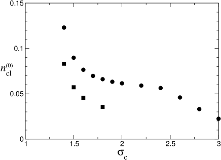
Figure 11: The variation of the gas cloud point density $n^{(0)}_{\rm cl}$ at $T=T_{c}$ as a function of $\sigma_{c}$, as obtained from MC simulations (squares) and MFE calculations (circles).

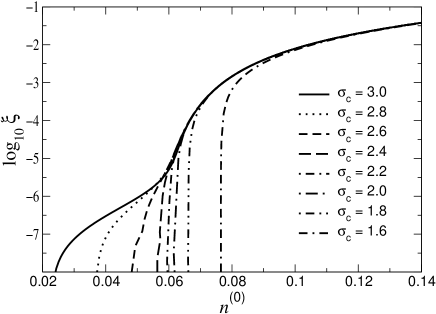
Figure 12: Plot of the fractional volume of the liquid phase versus parent density as predicted by the MFE theory at the critical temperature $t=t_{c}=0.437$. Results are displayed for a selection of size cutoffs as shown.

It is natural to enquire as to the conditions under which cutoff dependences can be expected be occur. The answer will, in general, depend on both the choice of the form of the parent size distribution $f^{(0)}(\sigma)$ and the size-dependence of the strength of the interaction between particles. It is straightforward to show SOLLICH02 that the density distribution of the liquid shadow phase is related to the parent via:

$$\rho^{\rm sh}(\sigma) = \rho^{(0)}(\sigma)\exp\left({-\beta[\mu^{\rm sh}_{\rm ex}(\sigma)-\mu^{\rm cl}_{\rm ex}(\sigma)]}\right)$$ (9)

$$\approx \rho^{(0)}(\sigma)\exp\left[{-\beta\mu^{\rm sh}_{\rm ex}(\sigma)}\right]$$ (10)

when the cloud point density is small. Thus when the excess activity $\exp[\beta\mu^{\rm sh}_{\rm ex}(\sigma)]$ in the shadow phase decreases faster with $\sigma$ than the corresponding decay in the parent size distribution, the shadow density distribution will be peaked at the cutoff.

We now analyse this scenario in more detail, for a more general size-dependence of the interaction strength, $\epsilon_{ij}=(\sigma_{i}\sigma_{j})^{\alpha}$. Our hypothesis is that, for suitable parent distributions $f^{(0)}(\sigma)$, the cloud point will move to vanishing density as the cutoff $\sigma_{c}$ is made large, while the corresponding shadow phase will consist only of particles with sizes close to $\sigma_{c}$. The shadow is then a scaled version of a “standard” (monodisperse, unit particle diameter) LJ system, but effectively at a temperature $T/\sigma_{c}^{2\alpha}$ because all interactions are stronger by a factor $(\sigma\sigma^{\prime})^{\alpha}\approx\sigma_{c}^{2\alpha}$; this effective temperature decreases to zero as $\sigma_{c}$ is made large. To coexist with the (infinitely, in the limit $\sigma_{c}\to 0$) dilute cloud phase, the shadow also has to be at zero pressure. At these zero temperature, zero pressure conditions, the shadow phase will be a crystalline solid, more precisely the ground state of the effectively monodisperse LJ system. To check that this scenario is self-consistent, we now need to work out the excess chemical potential $\mu_{\rm ex}^{\rm sh}(\sigma)$ of such a solid. It is convenient to use the Widom insertion expression $\exp[-\beta\mu_{\rm ex}^{\rm sh}(\sigma)]=\langle\exp(-\beta u_{\sigma})\rangle$; the average is over the position where the test particle of diameter $\sigma$ is inserted, uniformly over the whole system, and $u_{\sigma}$ is the interaction potential of this particle with all others. Given the assumed size-dependence of the interaction strength, we have $u_{\sigma}=(\sigma\sigma_{c})^{\alpha}u_{1}$, where $u_{1}$ is the interaction potential of a unit diameter test particle inserted into a standard LJ solid. Thus $\exp[-\beta\mu_{\rm ex}^{\rm sh}(\sigma)]=\langle\exp[-\beta(\sigma\sigma_{c})^{\alpha}u_{1}]\rangle$. When $\sigma_{c}$ is large, the average will be dominated by the minimum value $u_{1,\rm min}<0$ of $u_{1}$, i.e. the optimal insertion positions. Ignoring subexponential corrections then gives $\mu_{\rm ex}^{\rm sh}(\sigma)=-(\sigma\sigma_{c})^{\alpha}|u_{1,\rm min}|$. The excess chemical potential at $\sigma=\sigma_{c}$ thus scales as $\sigma_{c}^{2\alpha}$; looking at Eq. (10), the hypothesized cutoff-dominated shadow phase can then exist for parent size distributions decaying more slowly than $f^{(0)}(\sigma)\sim\exp(-{\rm const}\times\sigma^{2\alpha})$. Toward smaller $\sigma$, $-\mu_{\rm ex}^{\rm sh}(\sigma)\sim(\sigma\sigma_{c})^{2\alpha}$ decreases by an amount of $O(1)$ already for $\sigma_{c}-\sigma\sim\sigma_{c}^{1-2\alpha}\ll\sigma_{c}$. This fast decrease shows that also the assumption of a shadow size distribution sharply peaked towards $\sigma_{c}$ is self-consistent. For the particular case $\alpha=1$ studied in the rest of this paper, we have that the limiting parent size distribution where cutoff effects start to appear is Gaussian. The Schulz distribution has a substantially fatter (exponential) tail and it is therefore clear that cutoff dependences should arise, as observed.

As we have seen, the MFE results (cf. Fig. 10) predict that, as $\sigma_{c}$ is increased, so the shadow phase comprises ever more strongly interacting particles whose sizes are concentrated near $\sigma_{c}$. For large enough cutoffs, the general arguments advanced above show that this shadow phase must be a solid because it is effectively at very low temperature (as well as low pressure). Since the simple approximate free energy used for our theoretical predictions does not include a branch that could describe such solid phases, we have attempted to investigate this possibility via simulation. Unfortunately, owing to the computational burden of simulating systems with large cutoffs, we could not access the coexistence regime directly. We were, however, able to study the regime of metastable coexistence lying between the cloud curve and a system-size dependent “effective spinodal” BINDER03 . For large cutoffs, this region occurs at very low $n^{(0)}$, and accordingly one can, to a good approximation, assign the requisite chemical potential distribution on the basis of the value of the second virial coefficient, as described in Appendix A.

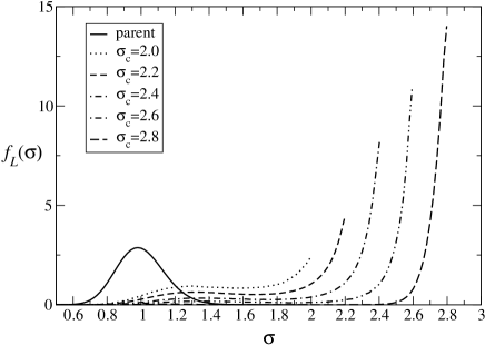
Figure 13: Size distribution $f_{L}(\sigma)$ in the metastable liquid phase for cutoffs in the range $\sigma_{c}=2.0$ to $\sigma_{c}=2.8$. Also shown for comparison is the parent form $f^{(0)}(\sigma)$.

Using this approach, we have studied the form of the size distribution in the metastable liquid daughter phase for a range of large cutoff values. The results in Fig. 13 show that, in accord with the MFE predictions, as $\sigma_{c}$ increases there is an accumulation of weight at $\sigma=\sigma_{c}$. Interestingly too, we find that for $\sigma_{c}=2.8$ the liquid spontaneously freezes to an f.c.c. crystal structure, as shown in Fig. 14. We emphasize that this occurs for $n^{(0)}$ values close to the effective spinodal point, not at the cloud point itself. However, given the above theoretical considerations it seems likely that, for $\sigma_{c}$ values larger than those presently accessible to direct simulation at the cloud point, the freezing will occur from the stable liquid phase SEAR .

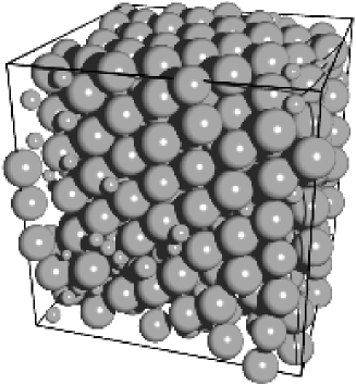
Figure 14: Snapshot configuration of the quasi-monodisperse metastable solid which coexists with the gas phase at $n^{(0)}=1\times 10^{-7}$ for $\sigma_{c}=2.8$.

In view of the likelihood of gas-solid coexistence at large $\sigma_{c}$ and small $n^{(0)}$, one can speculate as to the character of the overall phase diagram in this regime. One possibility is that depicted schematically in Fig. 15. Here on increasing $n^{(0)}$ from the stable gas region, at low $T$, the system reaches a gas-solid (GS) cloud point at which the gas splits off an infinitesimally small quantity of quasi-monodisperse solid. However, as more of this solid is formed it must become more polydisperse in order for the system overall to preserve the parent size distribution. Hence on further increasing $n^{(0)}$, the increasing polydispersity of the solid forces it to split off a liquid phase and the system must enter a region of gas-liquid-solid (GLS) coexistence. Finally, once all the solid has melted, there is a regime of gas-liquid (GL) coexistence, as is also seen for smaller cutoffs. It seems likely that at higher temperature the solid phase would not be stable, leading to a gas-liquid-solid triple point as shown.

Figure 15: Schematic representation of a possible phase diagram for large size cutoffs $\sigma_{c}$. The letters indicate the nature of the phases (G: gas, L: liquid, S: solid).

V Conclusions

In summary, we have deployed state-of-the-art MC simulation techniques and MFE calculations to study in detail the phase behaviour of a model fluid in which polydispersity affects both the particle sizes and the strength of their interactions. The latter aspect in particular is primarily responsible for a dramatic separation of cloud and shadow curves compared to a previous study of the purely size-disperse case WILDING04 . We have determined the cloud and shadow curves for our model, as well as the phase behaviour along certain dilution lines which span the coexistence region. We find that the locus of the cloud curve is acutely sensitive to the choice of the upper cutoff on the parent particle size distribution, even when this cutoff lies far in the tail of the distribution. Such effects imply that in experiments on polydisperse fluids (see e.g. ERNE05 ) it may be important to monitor and control carefully the tails of the size (or charge, etc) distribution. Otherwise undetected differences could lead to large sample-to-sample fluctuations in the observed phase behaviour.

The origin of the observed cutoff dependences has been traced to extremely pronounced fractionation effects, the nature of which we have elucidated in terms of the character of the size distribution of the shadow phase. We have also provided criteria for determining which combination of parent size distributions and interaction potentials can be expected to display cutoff effects. Our theoretical considerations, together with additional simulation evidence, suggest that, in the limit of very large cutoffs, the cloud point density tends to zero and new phases appear, such as a region of coexistence between a gas and a quasi-monodisperse crystal.

Finally, with regard to outstanding questions that have not been considered in the present work, we would highlight the nature of the critical behaviour. Specifically, nothing is known concerning the existence and nature of singularities in the cloud and shadow curves in the critical region, or indeed what constitutes a suitable choice of order parameter for characterizing the critical behavior. Intriguing experimental results on polydisperse polymers KITA suggest that the critical exponents are Fisher renormalized, though the reasons for this appear unclear at present. We hope to investigate these issues in future work.

Appendix A Virial estimate of chemical potential distribution at low parent density

For a monodisperse system, the chemical potential can be written to first order in the density as

$$\beta\mu_{\rm ex}=2\rho\sigma^{3}B_{2}^{\star}(T)$$ (A11)

with $B_{2}(T)$ the reduced second virial coefficient HANSEN .

For our polydisperse LJ potential, Eq. (3), this generalizes to

$$\beta\mu_{\rm ex}(\sigma)=2\int_{0}^{\sigma_{c}}\!\!d\sigma^{\prime}\,\rho(\sigma^{\prime})\left(\frac{\sigma+\sigma^{\prime}}{2}\right)^{3}B_{2}^{\star}(T/\sigma\sigma^{\prime})$$ (A12)

with

$$B_{2}^{\star}=-2\pi\int_{0}^{\infty}\!\!dr\,r^{2}\exp\left\{\frac{-4\sigma\sigma^{\prime}}{T}\left[\left(\frac{\bar{\sigma}}{r}\right)^{12}-\left(\frac{\bar{\sigma}}{r}\right)^{6}\right]-1\right\}$$

Numerical evaluation of the double integral in (A12) is simplified by noting that for the (untruncated) Lennard-Jones potential, $B_{2}^{\star}(T)$ can be expressed as a series:

$$B_{2}^{\star}(T)=\frac{-2\pi}{3}\sum_{n=0}^{\infty}\frac{1}{4n!}\left(\frac{4}{T}\right)^{(2n+1)/4}\Gamma\left(\frac{2n-1}{4}\right)$$ (A13)

with $\Gamma(z)$ the complete Gamma function. We have not corrected for the presence of a potential truncation.

- (1) R.G. Larson, The Structure and Rheology of Complex fluids (Oxford University Press, New York, 1999).
- (2) G.H. Fredrickson, Nature (London) 395, 323 (1998).
- (3) W.B. Russel, D.A. Saville and W.R. Schowalter, Colloidal Dispersions, (Cambridge U.P., Cambridge, 1989).
- (4) J.A. Gualtieri, J.M. Kincaid and G. Morrison, J. Chem. Phys. 77, 521 (1982).
- (5) For a review see: P. Sollich, J. Phys. Condens. Matter 14, R79 (2002).
- (6) R. M. L. Evans, D. J. Fairhurst, and W. C. K. Poon, Phys. Rev. Lett. 81, 1326 (1998).
- (7) R.M.L. Evans, Phys. Rev. E59 3192 (1999); J. Chem. Phys. 114, 1915 (2001).
- (8) A. van Heukelum, G.T. Barkema, M.W. Edelman, E. van der Linden, E.H.A de Hoog, R.H. Tromp, Macromolecules 36, 6662 (2003).
- (9) R. S. Shresth, R.C. McDonald, S.C. Greer, J. Chem. Phys. 117, 9037 (2002).
- (10) M.W. Edelman, E. van der Linden, R. H. Tromp, Macromolecules 336, 7783 (2003).
- (11) D.J. Fairhurst and R.M.L. Evans, Colloid & Polymer Science 282 766 (2004).
- (12) B. H. Erné, E. van den Pol, G.-J. Vroege, T. Visser and HH Wensink, Langmuir 21, 1802 (2005).
- (13) N.B. Wilding, M. Fasolo and P. Sollich, J. Chem. Phys. 121, 6887 (2004); N.B. Wilding and P. Sollich, Europhys. Lett. 67, 219 (2004).
- (14) J.J. Salacuse and G. Stell, J. Chem. Phys. 77, 3714 (1982).
- (15) R. Kita, K. Kubota and T. Dobashi, Phys. Rev. E 56, 3213 (1997).
- (16) M.R. Stapleton, D.J. Tildesley, N. Quirke; J. Chem. Phys. 92, 4456 (1990)
- (17) P.G. Bolhuis and D.A. Kofke, Phys. Rev. E54, 634 (1996); D.A. Kofke and P.G. Bolhuis, Phys. Rev. E59, 618 (1999).
- (18) D.A. Kofke; J. Chem. Phys. 98, 4149 (1993).
- (19) T. Kristóf and J. Liszi, Mol. Phys. 99, 167 (2001).
- (20) S. Pronk and D. Frenkel, Phys. Rev. E 69 066123 (2004).
- (21) M. A. Bates and D. Frenkel, J. Chem. Phys. 109, 6193 (1998)
- (22) N.B. Wilding, J. Chem. Phys. 119, 12163 (2003)
- (23) H. Xu and M. Baus, Phys. Rev. E61, 3249 (2000).
- (24) P. Sollich, P.B. Warren and M.E. Cates, Adv. Chem. Phys. 116, 265 (2001)
- (25) L. Bellier-Castella, H. Xu and M. Baus, J. Chem. Phys. 113, 8337 (2000).
- (26) A. Speranza and P. Sollich, J. Chem. Phys. 118, 5213 (2003).
- (27) N. Clarke, J.A. Cuesta, R. Sear, P. Sollich, and A. Speranza. J. Chem. Phys., 113, 5817 (2000).
- (28) A. Speranza and P. Sollich, J. Chem. Phys., 117, 5421 (2002).
- (29) M. Fasolo and P. Sollich, Phys. Rev. Lett. 91, 068301 (2003).
- (30) Y.V. Kalyuzhnyi and G. Kahl, J. Chem. Phys. 119, 7335 (2003).
- (31) Y.V. Kalyuzhnyi, G. Kahl and P.T. Cummings, J. Chem. Phys. 120, 10133 (2004).
- (32) C. Rascón and M.E. Cates, J. Chem. Phys. 118, 4312 (2003).
- (33) A short description of some aspects of this work has previously appeared elsewhere: N.B. Wilding, P. Sollich and M. Fasolo, Phys. Rev. Lett. 95, 155701 (2005).
- (34) G.V. Schulz. Z. Physik. Chem. B43, 25 (1939); B.H. Zimm, J. Chem. Phys. 16, 1099 (1948).
- (35) M. E. McDonnell, A. M. Jamieson, Journal of Applied Polymer Science 21 3261 (2003).
- (36) L. Kvitek et al, J. Mater. Chem 15, 1099 (2005).
- (37) N.B. Wilding and P. Sollich, J. Chem. Phys. 116, 7116 (2002). See also F. Escobedo, J. Chem. Phys. 115, 5642 (2001); ibid. 115, 5653 (2001).
- (38) M. Buzzacchi, P. Sollich, N.B. Wilding and M. Müller, Phys. Rev. E. 73, 046110 (2006). The method used in the present work was termed “method B” in this paper.
- (39) C. Borgs and W. Janke, Phys. Rev. Lett. 68, 1738 (1992); C. Borgs and R. Kotecky, Phys. Rev. Lett. 68, 1734 (1992).
- (40) A.M. Ferrenberg and R.H. Swendsen; Phys. Rev. Lett.63, 1195 (1989).
- (41) B. Berg and T. Neuhaus, Phys. Rev. Lett 68, 9 (1992).
- (42) N.B. Wilding; Am. J. Phys. 69, 1147 (2001).
- (43) T. Boublík, J. Chem. Phys. 53, 471 (1970).
- (44) G.A. Mansoori. N.F. Carnahan, K.E. Starling, T.W. Leland, J. Chem. Phys. 54, 1523 (1971).
- (45) N.B. Wilding, Phys. Rev. E52, 602 (1995).
- (46) K. Binder, Phys. Rev. A25, 1699 (1982).
- (47) K. Ŝolc, Macromolecules 8, 819 (1975).
- (48) M. Fasolo and P. Sollich, Phys. Rev. E 70, 041410, (2004).
- (49) K. Binder, Physica A 319, 99 (2003).
- (50) We note that in the limit of large polydispersities, freezing of polydisperse hard spheres into multiple fractionated solids is predicted to occur at arbitrarily low densities: R.P. Sear, Phys. Rev. Lett. 82, 4244 (1999). However the relationship of this phenomenon to the overall phase behaviour was not considered.
- (51) R. Kita, K. Kubota and T. Dobashi, Phys. Rev. E56, 3213 (1997); ibid 58, 793 (1998).
- (52) J.P. Hansen, I.R. MacDonald, Theory of Simple Liquids, Academic Press, New York (1986).