Aging and intermittency in a p-spin model of a glass

Abstract

We numerically analyze the statistics of the heat flow between an aging system and its thermal bath, following a method proposed and tested for a spin-glass model in a recent Letter (P. Sibani and H.J. Jensen, Europhys. Lett.69, 563 (2005)). The present system, which lacks quenched randomness, consists of Ising spins located on a cubic lattice, with each plaquette contributing to the total energy the product of the four spins located at its corners. Similarly to our previous findings, energy leaves the system in rare but large, so called intermittent, bursts which are embedded in reversible and equilibrium-like fluctuations of zero average. The intermittent bursts, or quakes, dissipate the excess energy trapped in the initial state at a rate which falls off with the inverse of the age. This strongly heterogeneous dynamical picture is explained using the idea that quakes are triggered by energy fluctuations of record size, which occur independently within a number of thermalized domains. From the temperature dependence of the width of the reversible heat fluctuations we surmise that these domains have an exponential density of states. Finally, we show that the heat flow consists of a temperature independent term and a term with an Arrhenius temperature dependence. Microscopic dynamical and structural information can thus be extracted from numerical intermittency data. This type of analysis seems now within the reach of time resolved micro-calorimetry techniques.

1 Introduction

Following the change of an external parameter, e.g.  a temperature quench, complex systems unable to re-equilibrate within observational time scales undergo a so-called aging process. During aging, physical quantities slowly change as a function of the time elapsed since the quench, a time conventionally denoted by the term ‘age’. In mesoscopic sized systems [1, 2] aging manifests itself through a sequence of large, so-called intermittent, configurational re-arrangements. These events generate non-Gaussian tails in the probability density function (PDF) of configurational probes such as colloidal particle displacement [3, 4] and correlation [5] or voltage noise fluctuations in glasses [6]. The intermittent signal contains valuable dynamical information which is straightforwardly collected in numerical simulations and which now seems within reach of highly sensitive calorimetric techniques [7].

The present work confirms the expected wider applicability of the method previously introduced in a Letter [8], and extends the analysis to include the temperature dependence of the rate of energy flow. Secondly, it features a more extensive discussion of record dynamics [9] as a paradigm for non-equilibrium aging and intermittency.

We consider the plaquette model [10, 11], which belongs to a class of Ising models with multiple spin interactions [10, 11, 12, 13, 14], known to possess central features of glassiness, e.g. a metastable super-cooled phase as well as an aging phase [10, 11].

In the sequel, a short summary is given of the relevant properties of the p-spin model and of the Waiting Time Algorithm [15] (WTM) used in the simulations. As a check of this algorithm, we calculate the known equilibrium and metastability properties of the model before turning to the heat flow analysis. We show that irreversible intermittent events, so called quakes, can be disentangled from the reversible and equilibrium-like fluctuations of zero average which occur around metastable configurations. The age and temperature dependences of the statistics of both types of events are described in detail. In the final section, our findings are summarized and placed in a broader context.

2 The model

We consider a set of $N=16^{3}$ Ising spins, $\sigma_{i}=\pm 1$, placed on a cubic lattice with periodic boundary conditions. The spins interact via the ‘plaquette’ Hamiltonian

$${\cal H}=-\sum_{{\cal P}_{ijkl}}\sigma_{i}\sigma_{j}\sigma_{k}\sigma_{l},$$ (1)

where the sum runs over all the elementary plaquettes of the lattice, each contributing the product of the four spins located at its corners.

By inspection, a ‘crystalline’ ground state of the model is the fully polarized state with energy per spin $\epsilon_{G}=-3$. Other ground states can be obtained by inverting the spins in any plane orthogonal to the $x$, $y$ or $z$ axes. These symmetries lead to a degeneracy $\approx 2^{3L}$, where $L$ is the linear lattice size.

The simulations of Lipowski and Johnston [10] show a disordered equilibrium state above $T\approx 3.6$, and, between $T=3.6$ and $T\approx 3.4$, the presence of a metastable ‘super-cooled liquid’ phase. According to Swift et al. [11] the energy autocorrelation function decays in this regime as a stretched exponential, with no age dependence. The duration of the metastable plateau diverges as $T\downarrow 3.4$. Below this temperature aging sets in.

3 The WTM algorithm

Monte Carlo algorithms reproduce central features of aging dynamics, and their use to study aging systems is thus empirically, if not rigorously, justified. As in ref. [8], the present simulations rely on the WTM [15], a rejectionless (event driven) MC algorithm [16], which obeys detailed balance. Unlike the Metropolis algorithm, the WTM relies on an intrinsic or ‘global’ time variable, which is akin to the clock time of a physical system, modulo an overall scale factor of little significance for aging behavior, where most quantities of interest depend on time ratios.

Let $b_{i}$ denote the energy change associated with the flipping of spin $i$ with fixed neighbors. For a given initial configuration, random waiting times $w_{i}$ are drawn from an exponential distribution with average $\tau_{i}=\exp(b_{i}/2T)$. A WTM move identifies the shortest waiting time, adds it to the ‘global’ time variable, and flips the corresponding spin. Spins whose $b$ values are affected by the current move have their waiting times recalculated. The others do not, since the statistical properties of their (memoryless) waiting process would be unchanged by a renewed evaluation. In unstable configurations, where negative $b_{i}$ values are present, the WTM generates short waiting times, leading to the nucleation of flip avalanches, which can be followed in detail. In Metropolis simulations, the spins considered for update are randomly selected, and events below the shortest time unit of one MC sweep cannot be resolved. Thus, while all MC algorithms with detailed balance converge, under weak conditions, to the same (Boltzmann) equilibrium state, they may do so in different ways, see e.g. ref. [17]. For our model, a comparison of the time dependence of the average energy to results previously obtained with the Metropolis algorithm only shows minor differences.

 

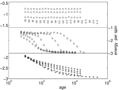
(a) Energy relaxation

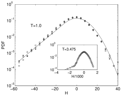
(b) Heat flow PDF

Figure 1: (a): The energy per spin is plotted vs. the system age for several temperatures, showing, from top to bottom, the presence of thermal equilibrium, metastability and aging. Data points are shown with symbols, the dotted lines are guides to the eye. In each panel, the temperatures corresponding to the five curves shown are, listed from top to the bottom: $T=4.75,4.25,3.75,3.57,3.50$ (upper panel), $T=3.475,3.45,3.40,3.25,3.00$ (middle panel) and $T=1.25,1.50,1.75,2.25,2.50$ (lower panel). (b): the PDF of the heat exchanged over an interval $\delta t$ at $T=1$ is sampled in the interval $[t_{w},3t_{w}]$. The three data sets shown have $t_{w}=300,1000$ and $5000$ respectively, with a fixed ratio $\delta t/t_{w}=0.01$. The insert shows similarly collected data for $t_{w}=5000$ and $T=3.475$. The line is a fit of the data to a function which equals an exponential for sufficiently negative $H$ value and a Gaussian for the rest of the range.

4 Results

Fig. 1(a) demonstrates the three known relaxation regimes of this model: For approximately $T\geq 3.500$, (top section), the energy immediately equilibrates at a high value. (The fast initial equilibration stage is omitted). In the interval $3.00<T<3.475$ (middle section), the final equilibrium near the ground state energy is reached after dwelling in a metastable plateau. The duration of the plateau grows with the temperature, reaching its maximum near $T=3.475$, i.e. near the temperature where metastability disappears. The equilibrium mean energy correspondingly undergoes an abrupt change between $T=3.475$ and $T=3.5$, in a way reminiscent of a first order transition[10]. At the low temperature end of the metastable regime, the plateau gradually softens, giving rise to a nearly logarithmic decay of the energy. Approximately below $T=2.50$ (bottom section) the energy value reached at any stage decreases with increasing temperature, an extreme non-equilibrium situation typical for the aging regime. In summary, the WTM and the Metropolis algorithm used in other works agree on the thermodynamical (average) behavior, with the hardly significant exception of the duration of the metastable plateau. The latter attains its maximum value at $T=3.40$ under the Metropolis update [11], and at a slightly higher temperature in the WTM case.

To investigate the energy flow statistics we choose a time interval $\delta t$ and partition the observation time $t$ into $[t/\delta t]$ intervals of equal duration. The heat $H$ exchanged over $\delta t$ arises as the difference between the energies of the two configurations at the endpoints of the interval,

$$H_{n}=E(t_{w}+(n+1)\delta t)-E(t_{w}+n\delta t),\quad n=1,2,\ldots[t/\delta t]$$ (2)

From ref. [8], we expect the rate of energy flow to fall off as $1/t_{w}$ (pure aging), leading to a $\delta t/t_{w}$ scaling of the PDF. For the present model, the collapse of three PDF’s shown in the main plot of Fig. 1, panel (b) confirms this expectation. The PDF’s are collected at $T=1.0$, i.e. deep in the aging regime, during time intervals $[t_{w},3t_{w}]$, with $t_{w}=300,1000$ and $5000$, (squares, diamonds and polygons, respectively), keeping the ratio $\delta t/t_{w}$ constant and equal to $0.01$. The insert shows data taken at $T=3.475$, i.e. at the upper edge of the metastable region. The calculations are repeated for $200$ independent trajectories, giving a total of $20000$ data points for each PDF.

The full line is a least square fit of the data to a continuous function comprising an exponential tail, $f_{<}(H)\propto e^{H/q}$ for $H<d<0$, and a Gaussian part centered at zero, $f_{>}\propto e^{-H^{2}/2{\sigma^{2}}_{rev}}$ for $H>d$. The position, $d$, of the joining point is itself a fitting parameter. As the overall scale of the PDF is arbitrary, the three parameters of physical significance are $q,\sigma_{rev}$ and $d$. Figure 1 (b) already indicates that the exponential intermittent tail carries the bulk of the energy flow. This also applies to the $T=3.475$ data shown in the insert, even though at this temperature, which is outside the aging regime, the intermittent events are swamped by the reversible Gaussian fluctuations.

 

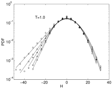
(a) Age dependence of intermittency

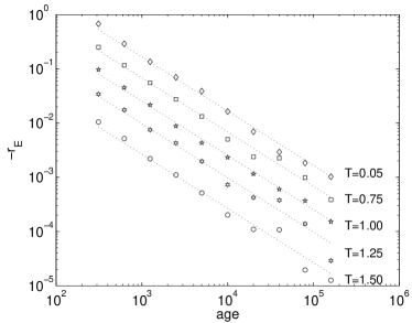
(b) Rate of energy flow

Figure 2: (a): The PDF of the heat exchanged between system and thermal bath over a time $\delta t=5$. Negative values correspond to an energy outflow. The data are based on $200$ independent runs, taken at temperature $T=1$ in the intervals $[t_{w},t_{w}+500]$ for $t_{w}=1000$ (diamonds), $t_{w}=2000$ (squares) $t_{w}=4000$ (polygons) $t_{w}=8000$ (hexagons) and $t_{w}=16000$ (circles). (b): The average rate of flow of the energy is plotted versus the age for the five temperatures shown. The full line has the form $y=ct_{w}^{-1}$, with the proportionality constant $c$ estimated as the mean of $t_{w}r_{E}$.

Further properties of the heat flow at $T=1$ are illustrated by panel (a) of Fig. 2. The five PDF’s shown are semilogarithmic plots of the distribution of $80000$ values of $H$ taken with $\delta t=5$. The values are sampled from $800$ independent trajectories, each stretching over an ‘observation’ interval of duration $t=500$.

For sufficiently negative $H$ values, all the PDFs have an exponential intermittent tail, which turns into a bell shaped, nearly Gaussian distribution as $H$ increases toward and beyond zero. The strongest intermittency observed in these data (top curve) is for $t_{w}=10^{3}$. Successively doubling $t_{w}$, up to $t_{w}=1.6\times 10^{4}$, leads to PDF’s approaching a Gaussian shape. This expresses the well known fact that aging systems appear equilibrated, when observed over a time shorter than their age. Importantly, the Gaussian part of the PDF has no conspicuous age dependence.

The full lines are, as mentioned, obtained as least square fits of the PDF data to a continuous, piecewise differentiable curve. The parameter $\sigma^{2}_{rev}$ estimates the variance of the reversible fluctuations and should not be confused with the full variance of $H$, which is mainly determined by the tail of the PDF.

The instantaneous rate of energy flow, a constant for time homogeneous dynamics, is here inversely proportional to the age. Ideally, this rate is obtained as the ensemble average of the ratio $\frac{H(\delta t,t_{w})}{\delta t}$, i.e.,

$$r_{E}(t_{w})\stackrel{{\scriptstyle{\rm def}}}{{=}}\lim_{\delta t\rightarrow 0}\frac{\langle H(\delta t,t_{w})\rangle}{\delta t}.$$ (3)

In practice we (mainly) use an ensemble of $1000$ independent trajectories, and perform in addition a time average over a finite observation interval $t$. We use $t=30$ for $t_{w}\leq 2500$, $t=100$ for $t_{w}\leq 40000$ and $t=500$ for $t_{w}>40000$. By varying $\delta t$ over the interval $[0.1,23]$ we ascertain that $\langle H\rangle$ is linearly dependent on $\delta t$. Finally, we estimate $r_{E}$ as the arithmetic average of $H(\delta t,t_{w})/\delta t$, over the approx. $5500$ data points available at each temperature. Panel (b) of Fig. 2 shows in a log-log plot the negative energy flow rate versus the system age, for five selected temperatures. To avoid clutter, the data sets belonging to each $T$ value are artificially shifted in the vertical direction by dividing, in order of increasing $T$, by $1,3,9,27$ and $81$. The full lines of Fig.2 are obtained by fitting the data to the form $r_{E}=c/t_{w}$, with the chosen value of $c$ minimizing the RMS distance to the data.

According to record dynamics [9, 8], the rate of quakes, $r_{q}$ obeys

$$r_{q}(t_{w})=\frac{\alpha(N)}{t_{w}},$$ (4)

where $\alpha$ represents the number of independent domains in the system, which is linearly dependent on the system size $N$, but independent of the temperature. The rate of energy flow depends on the rate of quakes and on the amount of energy given off in each quake. The latter could in principle depend on both temperature and age. However, since panel (b) of Fig. 2 shows that $r_{E}\propto 1/t_{w}$ to a good approximation, we conclude that $r_{E}(t_{w})=r_{q}(t_{w})e(T)$, where the average amount $e(T)$ of energy exchanged in a single quake is given by

$$e(T)=\frac{r_{E}\cdot t_{w}}{\alpha},$$ (5)

which only depends on $T$.

 

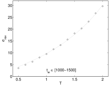
(a) Reversible fluctuations

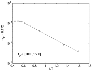
(b) Activated behavior of $r_{E}$

Figure 3: (a): The standard deviation $\sigma_{rev}$ of the reversible energy fluctuations is extracted from the Gaussian fit of the central part of the PDF data, and plotted versus the temperature. The dotted line is a fit to the theoretical prediction discussed in the main text. The data are based on $800$ independent runs, taken in the interval $[1000,1500]$. (b): The average rate of flow, shifted as indicated, is plotted logarithmically versus the inverse temperature. The straight line part of the data corresponds to Arrhenius activated behavior. These high precision data are based on $80000$ independent runs, all taken in the interval $[1000,1500]$.

Figure 3 covers the temperature dependence of the heat transport PDF in the age interval $[1000-1500]$. Specifically, panel (a) covers the $T$ dependence of the Gaussian part of the PDF, as described by the corresponding standard deviation $\sigma_{rev}$, while panel (b) covers the $T$ dependence of the intermittent tail, as described by the rate $r_{E}$.

In panel (a) the dots are the standard deviation $\sigma_{rev}$ of the reversible heat exchange fluctuations obtained from the Gaussian part of the PDF. The line is the theoretical prediction obtained under two model assumptions: (i) reversible energy fluctuations are treated as thermal equilibrium fluctuations, which (ii) occur independently within the previously introduced number $\alpha$ of thermalized domains. These are characterized by an exponential local density of states, ${\cal D}(e)\propto\exp(e/\epsilon)$. These assumptions lead, via standard thermal equilibrium calculations, to the expression

$$\sigma_{rev}=\surd(2\alpha)\frac{\epsilon T}{\epsilon-T};\quad T<\epsilon.$$ (6)

The parameter $\epsilon$ marks the upper limit of the temperature range where the exponential density of states is physically relevant (the attractor is thermally unstable and physically irrelevant for $T\geq\epsilon$). The pre-factor $\surd 2$ arises since $H$ is the difference of two energy values, taken $\delta t$ apart. These values are statistically independent, and the variance is correspondingly additive, provided that $\delta t$ is sufficiently large, as is the case here. Finally the pre-factor $\surd\alpha$ expresses the linear dependence of the variance on the number $\alpha$ of (supposedly) equivalent and independent domains. The parameter values minimizing the RMS distance between data and Eq. 6 are $\alpha=25$ and $\epsilon=3.8$. The domain volume corresponding to $\alpha=25$ is $v=16^{3}/25\approx 162$ spins, whence the linear size is, for a roughly cubic domain, close to $5$. The $\epsilon$ value is a theoretical upper bound to the thermal stability range, and safely exceeds $T=2.5$, the empirical upper temperature limit to the aging regime. Finally, using Eq. 5, the value $\alpha\approx 25$ and the available values of $r_{E}$, the average energy exchanged in a quake, $e(T)$, turns out to vary from $-8.8$ to $-15$ when $T$ varies from $0.65$ to $2.35$. In all cases $-e(T)>>T$, meaning that quakes are thermally irreversible on the time scale at which the occur, a necessary condition for record dynamics to apply [9, 8, 18]. In summary, the procedure just described seems preferable to e.g. a parabolic fit, which has nearly the same quality, but requires one more parameter, without providing a physical interpretation.

Panel (b) of Fig. 3 shows the temperature dependence of the energy flow rate $r_{E}$ in the age interval $[1000-1500]$. For fixed $t_{w}$ and $T\rightarrow 0$, $r_{E}$ approaches the value $\approx-0.172$. The logarithm of the deviation $-r_{E}-0.172$ is plotted in an Arrhenius fashion versus the reciprocal temperature $1/T$ (circles). The full line in panel (b) is an Arrhenius fit within the restricted range of $T$ obtained by excluding the lowest temperatures, as indicated. The fit yields an energy barrier of characteristic size $b\approx 3$. The modest activated contribution shows that once initiated, a quake can cover more ground the higher temperature, of course within the boundary of the aging regime. The activated contribution explains why, within a fixed amount of time, aging reaches lower energies at higher temperatures (see e.g. Fig. 1). In summary, the main contribution to the energy release is $T$ independent, but the process is nevertheless enhanced by an increased ability to climb small energy barriers.

5 Discussion

The heat exchange in the plaquette model features both equilibrium-like fluctuations, the Gaussian part of the PDF, and quakes, the exponential tail. Crucially, as the Gaussian signal has zero average, the energy outflow is exclusively due to the quakes, which we interpret [8, 9] as a change from one metastable configuration to another, having considerably lower energy. The interpretation is explicitely verified in a numerical study of the random orthogonal model [19], where energy changes from one inherent state (IS) [20] to another care monitored. The processes corresponding to the Gaussian and exponential parts of the PDF are there called stimulated and spontaneous, respectively.

As quakes are localized events in time and space, record dynamics treats aging as a strongly heterogeneous dynamical process. However, as emphasized by recent work [21, 22, 23, 24], exponential tails in the PDF’s of relevant dynamical variables also appear outside the aging regime (see also the insert of Fig. 1), i.e. heterogeneity is not exclusively associated to aging.

Our analysis employs a record dynamics scenario [9, 8], where quakes are assumed to be irreversible, an assumption appropriate far from equilibrium, and explicitely verified in the present model. The scenario has been used to design a numerical exploration technique [25, 26], melds, as we have seen, real space (the mumber $\alpha$ of domains) and ‘landscape’ (the density of states of local attractors) properties of glassy dynamics, and has a number of predictions which can be tested numerically and/or experimentally. The physical adjustments induced by each quake affect all measurements. In principle, these aspects require a separate modeling effort, which in our case is limited to the temperature dependence of the average energy $e(T)$ exchanged in a single quake. More generally, by assuming that the induced changes are stochastic and mutually independent, and that no rearrangement can occur without a quake, approximate closed-form expressions for the rate of change of any quantity of physical interest can be obtained [18, 27]. E.g., the configuration autocorrelation function and the linear response between times $t_{w}$ and $t_{w}+t$ are predicted to scale with the logarithm of the ratio $t/t_{w}$, as indeed observed [18, 28, 29] in a number of cases.

In the p-spin model, the average energy decays in logarithmic fashion, a behavior also seen in spin-glasses [8] and Lennard-Jones glasses [30]. In the latter case, the rate of hopping between different minima basins (arguably similar to our quakes, see also ref.[19] ) decreases as the reciprocal of the age. Broadly similar behavior is observed, experimentally or numerically, in a large number of other complex systems [31, 32, 33, 34].

Record dynamics sees aging as an entrenchment into a hierarchy of metastable attractors with growing degree of stability. It thus implies the existence of a hierarchy of the sort explicitely built into ‘tree’ models of glassy relaxation [35, 36, 37, 38, 39], models which notably reproduce key features of glassy dynamics. For such models, an entry in a hitherto unexplored subtree requires a record-sized energy fluctuation. The converse statement, which is assumed in record dynamics, is only true for a continuously branching tree, i.e. when the energy difference between neighboring nodes tends to zero. In spite of these mathematical difference, the physical picture behind record dynamics and tree models is nearly the same. Note that hierarchies are specifically associated to locally thermalized and independently relaxing real space domains. The fit in Fig. 3 simplistically assumes that, within each of these, the number of configurations available increases exponentially with the energy difference from the state of lowest energy within the domain. The same property is built in tree models, and leads [40] to a thermal instability when the temperature approaches from below the characteristic scale of the exponential growth ($\epsilon$ in our notation). Nearly exponential local density of states have been found by a variety of numerical techniques in a number of microscopic models [41, 42, 43, 44, 45, 46, 47], providing independent evidence of the physical relevance of the approximation.

In conclusion, intermittency data offer a unique window into the microscopic dynamics of aging systems, and open the possibility of investigating issues of central importance in the statistical physics of complex systems, e.g. barriers and attractor basins, using calorimetric experiments.

6 Acknowledgments

Financial support from the Danish Natural Sciences Research Council is gratefully acknowledged. The author is greatly indebted to Stefan Boettcher for suggesting this investigation and for his useful comments, and to Karl Heinz Hoffmann, Henrik J. Jensen and Christian Schön for discussions.

References

- [1] H. Bissig, S. Romer, Luca Cipelletti Veronique Trappe and Peter Schurtenberger. Intermittent dynamics and hyper-aging in dense colloidal gels. PhysChemComm, 6:21–23, 2003.
- [2] L. Buisson, L. Bellon and S. Ciliberto. Intermittency in aging. J. Phys. Cond. Mat., 15:S1163, 2003.
- [3] Willem K. Kegel and Alfons van Blaaderen. Direct observation of dynamical heterogeneities in colloidal hard-sphere suspensions. Science, 287:290–293, 2000.
- [4] Eric R. Weeks, J.C. Crocker, Andrew C. Levitt, Andrew Schofield and D.A. Weitz. Three-dimensional direct imaging of structural relaxation near the colloidal glass transition. Science, 287:627–631, 2000.
- [5] Luca Cipelletti, H. Bissig, V. Trappe, P. Ballesta and S. Mazoyer. Time-resolved correlation: a new tool for studying temporally heterogeneous dynamics. J. Phys.:Condens. Matter, 15:S257–S262, 2003.
- [6] L. Buisson, S. Ciliberto and A. Garciamartin. Intermittent origin of the large violations of the fluctuation dissipation relations in an aging polymer glass. Europhys. Lett., 63:603, 2003.
- [7] W. Chung Fon, Keith C. Schwab, ohn M. Worlock and Michael L. Roukes. Nonoscaled, phonon-coupled calorimetry with sub-attojoule/kelvin resolution. NANO LETTERS, 5:1968–1971, 2005.
- [8] P. Sibani and H. Jeldtoft Jensen. Intermittency, aging and extremal fluctuations. Europhys. Lett., 69:563–569, 2005.
- [9] Paolo Sibani and Jesper Dall. Log-Poisson statistics and pure aging in glassy systems. Europhys. Lett., 64:8–14, 2003.
- [10] A. Lipowski and D. Johnston. Cooling-rate effects in a model of glasses. Phys. Rev. E, 61:6375–6382, 2000.
- [11] Michael. R. Swift, Hemant Bokil, Rui D. M. Travasso and Alan J. Bray. Glassy behavior in a ferromagnetic p-spin model. Phys. Rev. B, 62:11494–11498, 2000.
- [12] Juan P Garrahan and M E J Newman. Glassiness and constrained dynamics of a short-range non-disordered spin model. Physical Review E, 62:7670, 2000.
- [13] Juan P. Garrahan Lexie Davison, David Sherrington and Arnaud Buhot. Glassy behavior in a 3-state spin model. J. Phys. A:Math. Gen, 34:5147–5182, 2001.
- [14] Marc Mezard. Statistical physics of the glass phase. Physica A, 306:25, 2002.
- [15] Jesper Dall and Paolo Sibani. Faster Monte Carlo simulations at low temperatures. The waiting time method. Comp. Phys. Comm., 141:260–267, 2001.
- [16] M. E. J. Newman and R. G. Palmer. Modeling Extinction. Oxford University Press, 2002.
- [17] A.T.J. Wang V. Gotcheva, Y. Wang and S. Teitel. Continuous-time monte carlo and spatial ordering in driven lttice gases: Application to driven vortices in periodic superconducting networks. Phys. Rev. B, 72:064505, 2005.
- [18] Paolo Sibani. Mesoscopic fluctuations and intermittency in aging dynamics. Europhys. Lett., 73:69–75, 2006.
- [19] A. Crisanti and F. Ritort. Intermittency of glassy relaxation and the emergence of a non-equilibrium spontaneous measure in the aging regime. Europhys. Lett., 66:253–259, 2004.
- [20] Frank H. Stillinger and Thomas A. Weber. Dynamics of structural transitions in liquids. Phys. Rev. A, 28:2408–2416, 1983.
- [21] P. Mayer, H. Bissig, L. Berthier, L. Cipelletti, J. P. Garrahan, P.Sollich and V. Trappe. Heterogeneous dynamics in coarsening systems. Phys. Rev. Lett., 93:115701, 2004.
- [22] G. A. Appignanesi and A. Montani. Mechanistic view of the relaxation dynamics of a simple glass-former. a bridge between the topographic and the dynamic approaches. Journal of Non-Crystalline Solids, 337:109–114, 2004.
- [23] Albert C. Pan, Juan P. Garrahan and David Chandler. Heterogeneity and growing length scales in the dynamics of kinetically constrained lattice gases in two dimensions. Phys. Rev. E, 72:1041106, 2005.
- [24] Juan P. Garrahan Mauro Merolle and David Chandler. Space-time thermodynamics of the Glass Transition. Proc. Natl. Acad. Sci. USA, 102:10837, 2005.
- [25] Jesper Dall and Paolo Sibani. Exploring valleys of aging systems : the spin glass case. Eur. Phys. J. B, 36:233–243, 2003.
- [26] Stefan Boettcher and Paolo Sibani. Comparing extremal and thermal explorations of energy landscapes. European Physical Journal B, 44:317–326, 2005.
- [27] Paolo Sibani, G.F. Rodriguez and G.G. Kenning. Intermittent quakes and record dynamics in the thermoremanent magnetization of a spin-glass. cond-mat/0601702, 2006.
- [28] Horacio E. Castillo, Claudio Chamon, Leticia F. Cugliandolo, José Luis Iguain and Malcom P. Kenneth. Spatially heterogeneous ages in glassy systems. Phys. Rev. B, 68:13442, 2003.
- [29] C. Chamon, P. Charbonneau, L. F. Cugliandolo, D. R. Reichman and M. Sellitto. Out-of-equilibrium dynamical fluctuations in glassy systems. J. Chem. Phys., 121:10120, 2004.
- [30] L. Angelani, R. Di Leonardo, G. Parisi and G. Ruocco. Topological description of the aging dynamics in simple glasses. Phys. Rev. Lett., 87:055502, 2003.
- [31] M. Lee P. Oikonomou, P. Segalova, T. F. Rosenbaum, A. F. Th. Hoekstra and P. B. Littlewood. The electron gas in a switchable mirror: relaxation, ageing and universality. J.Phys.:Condens. Matter, 17:L439–L444, 2005.
- [32] A. Hannemann, J. C. Schön, M. Jansen, and P. Sibani. Non-equilibrium dynamics in amorphous Si3B3N7. J. Chem. Phys., B 109:11770–11776, 2005.
- [33] L.P. Oliveira, Henrik Jeldtoft Jensen, Mario Nicodemi and Paolo Sibani. Record dynamics and the observed temperature plateau in the magnetic creep rate of type ii superconductors. Phys. Rev. B, 71:104526, 2005.
- [34] Alexander S. Balankin and Oswaldo Morales Matamoros. Devil’s-staircase-like behavior of the range of random time series with record-breaking fluctuations. Phys. Rev. E, 71:065106(R), 2005.
- [35] Paolo Sibani and Karl Heinz Hoffmann. Hierarchical models for aging and relaxation in spin glasses. Phys. Rev. Lett., 63:2853–2856, 1989.
- [36] K. H. Hoffmann and P. Sibani. Relaxation and aging in spin glasses and other complex systems. Z. Phys. B, 80:429–438, 1990.
- [37] P. Sibani and K.H. Hoffmann. Relaxation in complex systems : local minima and their exponents. Europhys. Lett., 16:423–428, 1991.
- [38] Y. G. Joh and R. Orbach. Spin Glass Dynamics under a Change in Magnetic Field. Phys. Rev. Lett., 77:4648–4651, 1996.
- [39] S. Schubert K.H. Hoffmann and P. Sibani. Age reinitialization in spin-glass dynamics and in hierarchical relaxation models. Europhys. Lett., 38:613–618, 1997.
- [40] S. Grossmann, F. Wegner, and K. H. Hoffmann. Anomalous diffusion on a selfsimilar hierarchical structure. J. Physique Letters, 46:575–583, 1985.
- [41] P. Sibani, C. Schön, P. Salamon, and J.-O. Andersson. Emergent hierarchical structures in complex system dynamics. Europhys. Lett., 22:479–485, 1993.
- [42] P. Sibani and P. Schriver. Phase-structure and low-temperature dynamics of short range Ising spin glasses. Phys. Rev. B, 49:6667–6671, 1994.
- [43] J. C. Schön and P. Sibani. Properties of the energy landscape of network models for covalent glasses. J. Phys. A, 31:8165–8178, 1998.
- [44] T. Klotz, S. Schubert, and K. H. Hoffmann. Coarse Graining of a Spin-Glass State Space. Journal of Physics-Condensed Matter, 10:6127–6134, 1998.
- [45] J. C. Schön and P. Sibani. Energy and entropy of metastable states in glassy systems. Europhys. Lett., 49:196–202, 2000.
- [46] J.C. Schön. The energy landscape of two-dimensional polymer. J. Phys. Chem. A, 106:10886–10892, 2002.
- [47] Sven Schubert and Karl Heinz Hoffmann. The structure of enumerated spin glass spaces. Comp. Phys. Comm., 17:191–197, 2005.