Study of the topological Hall effect on simple models

Abstract

Recently, a chirality-driven contribution to the anomalous Hall effect has been found that is induced by the Berry phase and does not directly involve spin-orbit coupling. In this paper, we will investigate this effect numerically in a two-dimensional electron gas with a simple magnetic texture model. Both the adiabatic and non-adiabatic regimes are studied, including the effect of disorder. By studying the transition between both regimes the discussion about the correct adiabaticity criterium in the diffusive limit is clarified.

I Introduction

When studying the Hall effect in ferromagnets, an anomalous contribution was found giving rise to a non-zero Hall effect even in the absence of an externally applied magnetic field. Spin-orbit coupling was invoked to explain this effect, as it gives rise to two scattering mechanisms (skew scattering Karplus ; Smit and side jump Berger ) leading to a preferential scattering direction that is different for spin-up and spin-down. Since the spin subbands in ferromagnets are unequally populated, this spin-dependent scattering can indeed give rise to a charge Hall effect in ferromagnets, while in normal semiconductors these mechanisms explain the much-discussed spin Hall effect Hirsch .

Quite recently, one has found that an anomalous Hall effect can exist even in the absence of spin-orbit interaction in some classes of frustrated ferromagnets like pyrochlore-type compounds with non-coplanar magnetic moments in the elementary cell Taguchi . In these systems, the Hall effect is a result of the Berry phase Berry an electron acquires when moving in a system with nontrivial (chiral) spin texture. Since the effect can be attributed to the topology of the magnetization field, the term topological Hall effect was coined Bruno . Theoretical calculations on this effect Ohgushi ; Nagaosa have mainly concentrated on the adiabatic regime, where the electron spin aligns perfectly with the local magnetization during its movement. In this regime, by doing a transformation that aligns the quantization axis with the local magnetization direction at every point in space, the original Hamiltonian can be mapped onto a model of spinless electrons moving in an effective vector potential Ohgushi ; Bruno . However, only a few papers have dealt with the non-adiabatic limit (using perturbation theory Tatara ) and even less is known about the transition between the two regimes.

In this paper, we will show numerical calculations on the topological Hall effect in a two-dimensional electron gas (2DEG). It was proposed that in this system an artificial chirality can be created e.g. by the stray field of a lattice of ferromagnetic nanocylinders placed above the 2DEG, having the advantage that all relevant parameters are controllable up to some extent Bruno . In the current paper however, we will only consider some very simple model chiralities in the system. Nevertheless, with these models we are able to investigate numerically the existence of the topological Hall effect. More importantly, the transition point between the non-adiabatic and adiabatic regime will be studied for different values of the elastic mean free path. In the diffusive regime, it is found that the transition occurs slower as we increase the amount of disorder. This sheds some light on a long-standing discussion about the relevant adiabaticity criterium; it is in agreement with the one derived by Stern Stern and speaks against the criterium put forward by Loss Loss .

The paper is subdivided as follows. In the next section, we will first give a more detailed description of the topological Hall effect, discussing the transformation of the original Hamiltonian in the adiabatic limit onto a model of spinless electrons moving in an effective vector potential. After different adiabaticity criteria are presented in section III, a discussion concerning the calculation of Hall resistances and resistivities follows. In particular, a special phase averaging method is introduced for describing large (i.e. system length $L$ $\gg$ phase coherence length $L_{\phi}$) disordered systems; technical details of this method are given in the appendix. The main results of the paper can be found in section V.

II Topological Hall Effect

In order to explain what the topological Hall effect is about, we will consider a two-dimensional electron gas (2DEG), subjected to a spatially varying magnetization $\mathbf{M}(\mathbf{r})$. The Hamiltonian of such a system can be written as:

$$H=-\frac{\hbar^{2}}{2m^{\ast}}\nabla^{2}-g\,\mathbf{\sigma}\cdot\mathbf{M}(\mathbf{r}),$$ (1)

with $m^{\ast}$ the effective electron mass, $\mathbf{\sigma}$ the vector of Pauli spin matrices, and $g$ a coupling constant. We assume that the amplitude of the magnetization is constant; only its direction is position dependent: $\mathbf{M}(\mathbf{r})=M\mathbf{n}(\mathbf{r})$, with $\mathbf{n}$ a vector of unit amplitude.

For our numerical purposes, it is necessary to obtain a tight-binding description of this system by discretizing the Schrödinger equation on a square lattice with lattice constant $a$. The tight-binding equivalent of Eq. (1) reads

$$H=-t\sum_{\langle ij\rangle}\sum_{\alpha}|i\alpha\rangle\langle j\alpha|-gM\sum_{i}\sum_{\alpha,\beta}|i\alpha\rangle\,\mathbf{\sigma}_{\alpha\beta}\cdot\mathbf{n}_{i}\,\langle i\beta|,$$ (2)

where $i,j$ label the lattice sites, $\alpha,\beta$ are spin indices, $t=\frac{\hbar^{2}}{2ma^{2}}$ is the hopping amplitude, and $\mathbf{n}_{i}=\mathbf{n}(\mathbf{r}_{i})$. The first summation runs over nearest neighbors.

When the coupling $g$ is large enough, the adiabatic limit is reached meaning that spin flip transitions will be absent and the electron spin will stay aligned to the local magnetization direction. In that case, the solutions for the spin-up spinors (with respect to the local magnetization) are given by

$$|\chi_{i}\rangle=\left(\begin{array}[]{l}\cos\left(\frac{\theta_{i}}{2}\right)\exp\left(-\mathrm{i}\frac{\phi_{i}}{2}\right)\\ \sin\left(\frac{\theta_{i}}{2}\right)\exp\left(\mathrm{i}\frac{\phi_{i}}{2}\right),\end{array}\right)$$ (3)

with $(\theta_{i},\phi_{i})$ the spherical coordinates of the local magnetization direction $\mathbf{n}_{i}$. By projecting the Hamiltonian onto the subspace spanned by these spinors, one can derive an effective Hamiltonian Anderson ; Ohgushi

$$H_{\text{eff}}=\sum_{\langle i,j\rangle}t^{\text{eff}}_{ij}|i\rangle\langle j|,$$ (4)

where the hopping amplitudes are now

$$t^{\text{eff}}_{ij}=-t\cos\left(\frac{\zeta_{ij}}{2}\right)\exp\left(\mathrm{i}\gamma_{ij}\right).$$ (5)

In this expresssion, $\zeta_{ij}$ is the angle between the vectors $\mathbf{n}_{i}$ and $\mathbf{n}_{j}$. The angle $\gamma_{ij}$ needs some more explanation. Suppose an electron makes a closed trajectory around a lattice cell like depicted in Fig. 1. Since its spin follows adiabatically the local magnetization direction, the electron will pick up a Berry phase that is equal to half the solid angle $\Omega$ subtended by the magnetization directions at the four corners of the cell Berry , and the quantity $\gamma_{ij}$ is related to this Berry phase.

To make things more clear, let’s consider a flux

$$\Phi/\Phi_{0}=\frac{\Omega}{4\pi}$$ (6)

piercing through a lattice cell and forget about the magnetization for a moment ($\Phi_{0}=h/e$ is the magnetic flux quantum). The influence of such a fluxtube can be described in a tight-binding model by a Peierls substitution, Peierls which would change the hopping phase as $t\rightarrow t\exp(-\mathrm{i}e/\hbar\int\mathbf{A}\cdot\mathrm{d}\mathbf{l})$, with the integral evaluated along the hopping path. This is similar to the phase factor in Eq. (5) with

$$\gamma_{ij}=-e/\hbar\int_{i}^{j}\mathbf{A}\cdot\mathrm{d}\mathbf{l},$$ (7)

meaning that in principle the Berry phase effect can be described by an effective vector potential. E.g., one could make a choice of gauge for $\mathbf{A}$ such that the hopping phase on all the vertices above the fluxtube change as $t\rightarrow t\exp\left(\mathrm{i}2\pi\Phi/\Phi_{0}\right)=t\exp\left(\mathrm{i}\Omega/2\right)$ (see Fig. 1). This gauge choice would correspond to the Landau gauge in a situation where the effective fluxes through all lattice cells would be equal (i.e. there is a homogeneous field). In short, the effect of the $\gamma_{ij}$ can thus be described by having a distribution of effective magnetic fluxes piercing through the lattice cells. As such, for a given gauge, the quantities $\gamma_{ij}$ are defined in a unique way.

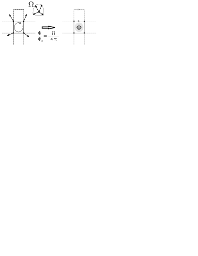
Figure 1: Mapping of the tight-binding Hamiltonian for an electron in a magnetic texture to a spinless electron moving around a fluxtube. Grey color of the vertices on the right picture stand for the change in hopping amplitude, while the arrows denote a change in hopping phase due to the fluxtube.

In summary, the effect of the transformation on the tight-binding Hamiltonian will be twofold: first, the hopping amplitude between neighbors changes, depending on the angle between the magnetization directions, and secondly, there is a Berry phase effect that effectively can be described in terms of a fluxtube distribution, where the value of the flux (in units $\Phi_{0}$) through a single lattice cell is given by $\frac{\Omega}{4\pi}$, and $\Omega$ is the solid angle subtended by the magnetization directions at the four corners of the lattice cell.

By means of this mapping it is clear now that the magnetization texture can indeed give rise to a Hall effect. It should be noted that the effective flux is given by a solid angle, so that the topological Hall effect can only be nonzero for non-coplanar textures. Furthermore, there is no need to invoke any kind of spin-orbit coupling for the topological Hall effect to appear.

III Adiabaticity Criterium

In order to be able to do the transformation between the Hamiltonian describing an electron moving in a magnetization texture [Eq. (1), which will be referred to as the magnetization model from now on], and the effective Hamiltonian in Eq. (4) [called the flux model from now on], the electron spin has to stay aligned to the local magnetization direction during its movement. This adiabatic regime will be reached when the spin precession frequency $\omega_{s}$ is large compared to the inverse of a timescale $\tau$ that is characteristic for the rate at which the electron sees the magnetization direction change.

If transport through the nanostructure is ballistic (i.e. there is no disorder), then this timescale is given by $\tau=\xi/v_{F}$, where $v_{F}$ is the Fermi velocity of the electrons, and $\xi$ is the length scale over which the magnetization changes its direction substantially. In this case, the adiabaticity criterium is thus

$$Q=\frac{\omega_{s}\xi}{v_{F}}\gg 1.$$ (8)

When introducing disorder in the system, it is clear that this criterium is still valid as long as the mean free path $l_{m}$ is larger than $\xi$. However, when going to the strongly diffusive regime $l_{m}<\xi$, two different timescales $\tau$ appear in the literature and there is still a discussion going on about the relevant one. Stern ; Loss ; Popp ; vanLangen In analytical calculations on rings, Stern has found that the relevant timescale would be the elastic scattering time $\tau=\tau_{m}$, leading to what is referred to as the pessimistic criterium in the literature Stern

$$Q\gg\frac{\xi}{l_{m}}.$$ (9)

However, other papers by Loss and coworkers Loss have put forward that the relevant timescale is the Thouless time $\tau_{\text{th}}=(\xi/l_{m})^{2}\,\tau_{m}$, i.e. the time the particle needs to diffusive through a distance $\xi$. This would lead to a less stringent adiabaticity criterium since $\tau_{\text{th}}>\tau_{m}$ in the diffusive regime, and it is therefore known as the optimistic criterium:

$$Q\gg\frac{l_{m}}{\xi}.$$ (10)

In a paper of van Langen et al. the pessimistic criterium was confirmed by a semi-classical analysis vanLangen , and later numerically by Popp et al. Popp In section V, we will have a closer look at the transition point between the adiabatic and non-adiabatic regimes ourselves and find also confirmation for the criterium in Eq. (9).

IV Calculation of the Hall resistance

In order to observe the topological Hall effect, we will numerically calculate the Hall resistance in a geometry like shown in Fig. 2. The Hall resistance $R_{H}$ in this geometry is defined as

$$R_{H}=\frac{1}{2}(R_{12,34}-R_{34,12}),$$ (11)

where we use the common notation

$$R_{ij,kl}=\frac{V_{k}-V_{l}}{I_{i}}$$ (12)

for a measurement where current is supplied through contacts $i$ and $j$, and the voltage difference $V_{k}-V_{l}$ is measured, fixing $I_{k}=I_{l}=0$. Making the difference between these two four-point resistances is equivalent to defining the Hall resistivity $\rho_{H}=\frac{1}{2}(\rho_{xy}-\rho_{yx})$ as the part of the resistivity tensor that is anti-symmetric with respect to time reversal Buettiker .

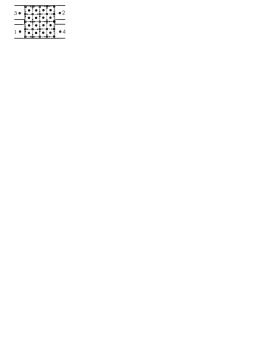
Figure 2: Geometry of a single section used to calculate the Hall resistance. A possible magnetization texture is shown. In the leads, the magnetization is chosen to point out of the plane of the paper.

Within the Landauer-Büttiker (LB) formalism, the four-point resistances in Eq. (12) can be expressed as Buettiker

$$R_{ij,kl}=\frac{h}{e^{2}}\frac{T_{ki}T_{lj}-T_{li}T_{kj}}{D}$$ (13)

as a function of transmission probabilities $T_{pq}$ between the leads. In this expression, $D$ is an arbitrary $3\times 3$ subdeterminant of the matrix $A$ relating the currents and the voltages on the leads: $I_{p}=\sum_{q}A_{pq}V_{q}$.

In principle, one could proceed now by calculating $R_{H}$ as a function of the adiabaticity parameter $Q$ and compare the rate of convergence for samples with different mean free paths in order to find the relevant adiabaticity criterium in the diffusive regime. However, since we make use of the LB-formalism, it is assumed that the whole structure is phase coherent. It is well known that the resistances in such structures are quantitatively strongly dependent on the actual configuration of the impurities in the system even when they are characterized by the same mean free path. Although this is an integral part of the physics of mesoscopic systems, it makes a quantitative comparison of $R_{H}$ between samples with different mean free paths useless. We would like to compare properties of a macroscopic system, i.e. a system with a finite phase coherence length in which such fluctuations are absent.

Therefore, some kind of (phase) averaging over different disorder configurations has to be introduced to find a description of the transport properties in terms of a macroscopic material constant, like the Hall resistivity. Some care should be taken in defining such an averaging procedure; e.g., just calculating the mathematical average $R_{H}=\frac{1}{N}\sum_{i=1}^{N}R_{H}^{i}$ of the Hall resistances $R_{H}^{i}$ found for $N$ different impurity configurations does not give a quantity that is directly related to the Hall resistivity $\rho_{H}$ of a macroscopic system.

The basic idea behind the averaging procedure we have chosen is that a macroscopic system ($L\gg L_{\phi}$) can be thought to consist of smaller phase coherent sections of size $L\approx L_{\phi}$. For every smaller section, we can use the LB-formula to derive its transport properties, and the properties of a macroscopic system can then be found by attaching such sections in an incoherent way. In our case, the smaller sections from which a macroscopic system will be built up are structures with the geometry in Fig. 2. Since a more detailed discussion of our particular averaging procedure and the corresponding Hall resistivity $\rho_{H}$ is rather technical, it is given in a separate appendix at the end of the paper.

V Results

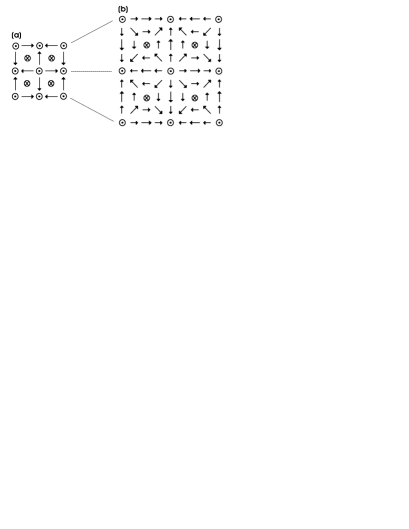
Figure 3: Basic cell for the texture of the magnetization (a). Every arrow corresponds to the magnetization direction at a single lattice site. By scaling up once, a more smoothly varying magnetization texture is obtained, resulting in smaller solid angles subtended by a single lattice cell (b). In (a) all arrows lie in the plane of the paper, while in (b) the magnetization is shown projected onto this plane: smaller arrows mean a shorter projection.

Before discussing the main results of the paper, a few words should be said about the model we have chosen for the magnetic texture in our numerical calculations. We started from a $4\times 4$ cell like depicted in Fig. 3a. Only the direction of the magnetization changes from site to site like depicted in the figure, while its magnitude stays constant. However, when mapping this texture to a flux model (like described in section II), one finds that the $4\times 4$ cell comprises a total flux of $4\,\Phi_{0}$, corresponding to an effective flux per lattice cell of $\Phi=1/4\Phi_{0}$, which is quite large. One could decrease this value by decreasing the solid angle subtended by the magnetization direction vectors at the corners of each lattice cell, since the flux per lattice cell is proportional to it [see Eq. (6)]. In order to do so one can scale up the cell of Fig. 3a by introducing extra lattice sites in between the original sites, and by interpolating the magnetization direction at the new sites between the directions of the neighboring sites. Scaling up the cell of Fig. 3a once, one then finds a magnetization cell of $8\times 8$ sites, like depicted in Fig. 3b. Of course the total flux comprised by this cell is still $4\,\Phi_{0}$, but this time distributed over $64$ sites, which corresponds to an average flux per lattice cell of $1/16\,\Phi_{0}$. This magnetizion cell can then in turn again be scaled up; every time we scale up the cell, it will comprise 4 times the original number of sites so that the average flux per lattice cell will be decreased by four. It should be noted that although the effective flux per lattice cell for the $4\times 4$ magnetization unit cell we started from is homogeneously distributed (exactly $1/4\,\Phi_{0}$ per lattice cell), this is not anymore the case for the cells found by scaling up the first one.

As a first step, we will have a look at a small sections with the geometry in Fig. 2. In the rest of the paper, we will model these sections by a tight-binding lattice comprising $65\times 65$ sites. The leads connected to them have a width of $30$ sites. The magnetization in the leads connected to the sample is chosen to point out of the plane of the paper on every site. When translating this to the flux model, it means that there is zero magnetic flux per lattice cell in the leads. In the device itself, a magnetization cell of $16\times 16$ sites is used, found from scaling up the original cell in Fig. 3a two times. We can fit $16$ such magnetization cells in one of our $65\times 65$ samples.

Figure 4: Hall resistance as a function of energy for a single section with magnetization texture obtained by scaling up the cell in Fig. 3a twice.

In Fig. 4, we have calculated the Hall resistance $R_{H}$ as defined in Eq. (11) for a single structure like depicted in Fig. 2, and for energies of the incoming electrons ranging from $0$ up to $2\,t$ above the bottom of the spin up band. The spin splitting due to the magnetization was chosen as large as $\Delta=gM=100\,t$, making sure that we are in the adiabatic regime (no disorder is present in the system). The results clearly show a nonzero Hall resistance $R_{H}$; in fact, one can clearly observe the integer quantum Hall effect. This indeed proves that a Hall effect is present although we do not have any magnetic flux present, nor any kind of spin-orbit coupling. The topological Hall effect seen here is purely due to the Berry phase an electron picks up when moving through a structure with a magnetization texture with nonzero spin chirality.

As explained in section II, one can map the model with the magnetization texture to a spinless flux model. For the magnetization texture we have chosen, the effective average flux per lattice cell will be $\Phi/\Phi_{0}=1/64$. This corresponds to a cyclotron radius of $10\,a$ (for the Fermi energy $E_{F}=1\,t$), which is much smaller than the sample size so that the integer quantum Hall effect could indeed be expected. When doing the mapping onto the flux model by calculating the effective hopping parameters like in Eq. (5) for our particular choice of magnetization texture, and then calculating the Hall resistance $R_{H}$, we found indeed perfect overlapping between the resistances of the two models. It can be claimed that the perfect overlap between the two models does not come as a surprise because in the quantum Hall regime the Hall resistance is quantized into exact plateaus. However, calculations were done even outside the quantum Hall regime, and the overlap between the two models is always exact within our numerical accuracy. Furthermore, the main point here is the fact that a Hall effect can be observed that is due to the electron adiabatically following a certain magnetization structure, and this is clearly demonstrated by Fig. 4.

Now that the topological Hall effect has been demonstrated numerically, we can proceed to study the transition from the non-adiabatic to the adiabatic regime. This will be done as a function of disorder strength (mean free path), in order to check which of the two adiabaticity criteria in section III are correct. As disorder is introduced in the system (within the Anderson model), a phase averaging procedure like set out in the previous section (and described fully in the appendix) has to be done in order to get quantitative information. For every separate value of the mean free path, we have calculated the transmission coefficients for $500$ small sections (Fig. 2) with different impurity configurations. Then we have wired together $4900$ sections randomly chosen from these $500$ in a square $70\times 70$ array, and calculated the resistivity of the obtained structure like described in the appendix (Fig. 7d). For the magnetization texture, we have chosen a $64\times 64$ cell found by scaling up the cell in Fig. 3a three times. A single section thus comprises a single cell of the magnetization. The shortest distance over which the magnetization changes its direction by an angle $\pi$ is given by $\xi\approx 22\,a$ for this particular cell. The Fermi energy was fixed to $E_{F}=1\,t$ above the bottom of the spin up subband.

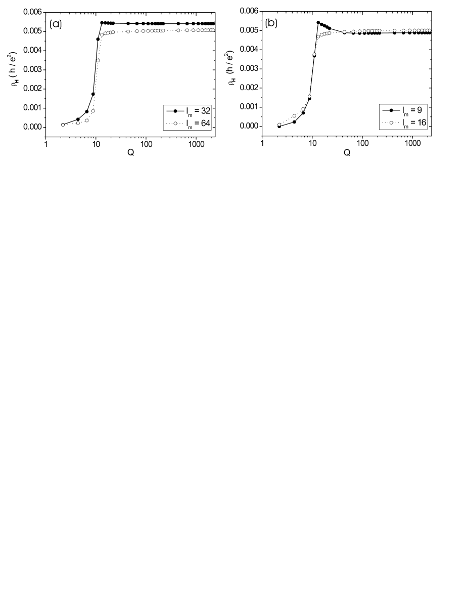
Figure 5: Hall resistivity as a function of the adiabaticity factor $Q$ for different values of the mean free path.

Fig. 5a shows the Hall resistivity $\rho_{H}$ defined in Eq. (17) for mean free paths $l_{m}=32\,a$ and $l_{m}=64\,a$, as a function of the adiabaticity parameter $Q=\omega_{s}\xi/v_{F}=\hbar\Delta\xi/v_{F}$. For both values of the mean free path the adiabatic limit is reached simultaneously for values of $Q\approx 20$, where the Hall resistivity becomes independent of $Q$. This is in good agreement with the adiabaticity criterium in Eq. 8. Furthermore, it was checked that the adiabatic value of the Hall resistivity coincides with the one calculated by mapping the magnetization model to the flux model. It should also be noted that $\rho_{H}$ is independent of the mean free path ($\rho_{H}\approx 5\times 10^{-3}\,\frac{h}{e^{2}}$) which is essentially what one might expect from a simple Drude model. Another feature on the figure is that $\rho_{H}$ does not increase linearly for small $Q$; instead it stays very small up to some point where it changes abruptly. This point coincides with a value for the spin splitting $\Delta=E_{F}$. Thus adiabaticity is reached on a rather short scale as soon as the Fermi energy lies below the spin down subband.

Figure 5b shows the same plot, but now for mean free paths in the diffusive regime ($l_{m}<\xi$), namely $l_{m}=9\,a$ and $l_{m}=16\,a$. Again, the Hall resistivity increases abruptly around $Q\approx 20$ to its adiabatic value. The resistivity $\rho_{H}$ obtains again the same value as in Fig. 5a around $\rho_{H}\approx 5\times 10^{-3}\,h/e^{2}$ and is thus clearly independent of the mean free path. Although $\rho_{H}$ changes abruptly, it can be seen that the real adiabatic value is reached slower for the lower of the two mean free paths ($l_{m}=9\,a$) for which $\rho_{H}$ first overshoots its adiabatic value, and then slowly converges to it. This difference is made more visible in Fig. 6, where we plotted the difference between the Hall resistivity $\rho_{H}$ and the adiabatic value it reaches (so that all curves converge to 0), for mean free paths of $l_{m}=9\,a,12\,a$ and $16\,a$. Again, it is clear that increasing the amount of disorder leads to a slower convergence to the adiabatic regime. As such, we confirm that the pessimistic adiabaticity criterium, which states that adiabaticity is reached more slowly upon decreasing the ratio $l_{m}/\xi$ [see Eq. (9)], is the correct one. Although for our limited range of allowed parameters (we should have $l_{m}>\lambda_{F}$ so that localization effects do not start playing a role) both adiabaticity criteria do not differ very much quantitatively, $Q\gg 0.45$ versus $Q\gg 2$ for $l_{m}=9\,a$, the optimistic criterium would predict the opposite behavior.

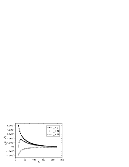
Figure 6: Hall resistivity as a function of the adiabaticity factor $Q$ in the intermediate regime. Decreasing the mean free path leads to a slower convergence to the adiabatic value. All plots are shifted so as to converge to $0$.

VI Conclusions

In this paper, we have shown numerical calculations confirming the existence of a fully topological Hall effect, that is due to the Berry phase an electron picks up when moving adiabatically in a non-coplanar magnetization texture. In the adiabatic regime, the governing Hamiltonian can be mapped onto a model of spinless electrons moving in a magnetic flux; both models indeed give the same results for the Hall resistance/resistivity. A closer look at the transition point between non-adiabatic and adiabatic regime revealed a rather abrupt transition upon increasing the exchange splitting. The transition takes place around the point where the spin-down subband becomes depopulated. Furthermore, we were able to find confirmation for the pessimistic adiabaticity criterium Stern by looking at the transition point for different mean free paths in the strongly diffusive regime. In this regime, a special method for phase averaging should be introduced for getting rid of conductance fluctuations, which enables us to describe the transport properties of a large system ($L>L_{\phi}$) in terms of a Hall resistivity.

Appendix A Phase averaging procedure

The main idea behind our averaging procedure is that a macroscopic system can be built up from smaller phase coherent subsections that are attached in an incoherent way. The small sections we would like to start from were depicted in Fig. 2. However, there is a subtle point that should be considered first: it is known that at every interface between a lead and the electron reservoir feeding this lead, a so-called contact resistance is present (see e.g. Imry and references cited there). Essentially such contact resistance results because on one side (the reservoir) current is carried by an infinite number of modes, while on the other side (the mesoscopic lead) there are only a finite number of modes transporting current. When building up a system of macroscopic size from the smaller sections, such contact resistance effects in the current-voltage relations of a single section are unwanted since they are characteristic of the leads, and not the sample itself.

In order to get rid of contact resistance effects, we will make an eight-terminal structure by attaching four extra voltage probes as in Fig. 7a. Since these extra voltage probes do not draw any current, there will be no voltage drop over their contact resistances, and they will measure the voltage at the point where they are attached. Placing them like in Fig. 7a, one is able to measure the voltage drops over the sample, excluding the voltage drops over the contact resistances of the original four current carrying leads (Fig. 7b). Relating now the currents through the original leads to the voltages measured with the voltage probes, one gets rid of the contact resistance effects.

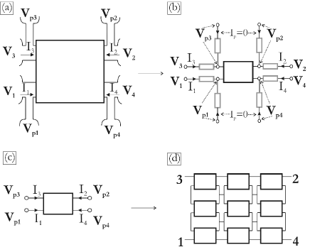
Figure 7: Scheme of the phase averaging procedure. Four extra voltage probes are attached to the original four-terminal structure (a). At every reservoir/lead interface a contact resistance is present; these are depicted in grey in (b). Since the voltage probes do not draw current, they will measure voltage drops over the sample, not including the contact resistances. Every section can now be considered as an effective four-terminal box characterized by a set of equations between currents through the original four leads, and the voltages measured by the extra voltage probes (c). Such boxes are wired up to form a macroscopic system, and its resistivities can be found by the van der Pauw technique (d).

Formally, this can be done with the Landauer-Büttiker formalism as follows. First we write down a set of linear equations relating the currents and voltages at all eight leads:

$$\left[\begin{array}[]{c}\mathbf{I}\\ \mathbf{I_{p}}\end{array}\right]=\left[\begin{array}[]{cc}A&B\\ C&D\end{array}\right]\left[\begin{array}[]{c}\mathbf{V}\\ \mathbf{V_{p}}\end{array}\right],$$ (14)

where $\mathbf{I}=(I_{1},\ldots,I_{4})$ is a vector containing the currents through the original four terminals, and $\mathbf{I_{p}}=(I_{p1},\ldots,I_{p4})$ are the currents through the voltage probes; the same notation convention is used for the voltages on the leads. The $4\times 4$ matrices $A,B,C$ and $D$ consist of transmission coefficients between all eight leads, and are found directly from the Landauer-Büttiker equations.

Since the voltage probes do not draw current, we find

$$\mathbf{I_{p}}=0=C\mathbf{V}+D\mathbf{V_{p}},$$ (15)

which can be used to express the currents through the four current-carrying leads as a function of the voltage on the attached voltage probes:

$$\mathbf{I}=\big{[}B-AC^{-1}D\big{]}\mathbf{V_{p}}.$$ (16)

Doing so, we have found current-voltage relations for the original four-terminal structure, but since we relate currents through the original leads to voltages at the voltage probes, we have gotten rid of contact resistances.

Subsequently, a large number of such structures (with different impurity configurations) are wired together as shown in Fig. 7d. Every single section is treated as a classical four-terminal circuit obeying current-voltage relationships of the form (16) [see also Fig. 7c]. Doing so, we introduce an effective phase breaking event at every connection point between neighboring sections: only current and voltage information is kept at these points, and any phase information of electrons flowing out of the section is lost. In other words, an artificial phase coherence length $L_{\phi}$ corresponding to the length of a single small section is introduced in the system.

By applying the correct current conservation laws at the intersection points in Fig. 7d, one can derive a relationship between the currents and voltages on the four terminals at the corners of the connected structure (labeled 1 to 4 in the Fig. 7d). When enough sections are attached, this relationship will be independent of the impurity configurations in the isolated sections. The properties of the system can then be expressed in terms of resistivities by making use of the van der Pauw technique vanderPauw . First, the four-terminal resistances $R_{12,34},R_{34,12},R_{14,23}$ and $R_{42,31}$ between the corners of the large structure are calculated. With these, the Hall resistivity is defined by vanderPauw ; Janecek

$$\rho_{H}=R_{H}=\frac{1}{2}(R_{12,34}-R_{34,12})$$ (17)

while the longitudinal resistivity $\rho_{L}$ can be found from solving the equation vanderPauw

$$\exp\left(-\pi R_{14,23}/\rho_{L}\right)+\exp\left(-\pi R_{42,31}/\rho_{L}\right)=1$$ (18)

A small comment should be made here. Because of the attachment procedure described above, one cannot expect the resistivities calculated in Eqs. (17) and (18) to correspond exactly to the real resistivities of a ”bulk” system of the same size and with the same mean free path; in particular, the resistivities as calculated above depend on the width of the leads attached to the small sections that make up the large system, and also on the scheme of wiring the sections together. In theory one could take into account these effects (see e.g. Ref. vanderPauw, ), and one would find that the real “bulk” resistivity and the resistivity calculated above are equal up to a factor that is purely geometrical. Calculating this factor explicitly is practically quite difficult; we did not proceed in this direction since the factor is of a purely geometric origin and has no physical implications.

References

-
(1)
R. Karplus and J. M. Luttinger, Phys. Rev. 95, 1154
(1954)
J. M. Luttinger, Phys. Rev. 112, 739 (1958). - (2) J. Smit, Physica (Amsterdam) 24, 39 (1958).
- (3) L. Berger, Phys. Rev. B 2, 4559 (1970); ibid. 5, 1862 (1972).
- (4) J. E. Hirsch, Phys. Rev. Lett. 83, 1834 (1999).
-
(5)
Y. Taguchi, Y. Oohara, H. Yoshizawa, N. Nagaosa, and Y. Tokura,
Science 291, 2573 (2001).
Y. Taguchi, and Y. Tokura, Europhys. Lett. 54, 401 (2001). - (6) M. V. Berry, Proc. R. Soc. London A 392, 45 (1984).
- (7) P. Bruno, V. K. Dugaev, and M. Taillefumier, Phys. Rev. Lett. 93, 096806 (2004).
- (8) K. Ohgushi, S. Murakami, and N. Nagaosa, Phys. Rev. B 62, R6065 (2000).
- (9) S. Onoda, and N. Nagaosa, Phys. Rev. Lett. 90, 196602 (2003).
-
(10)
G. Tatara, and H. Kawamura, J. Phys. Soc. Jpn. 71, 2613
(2002).
M. Onoda, G. Tatara, and N. Nagaosa, J. Phys. Soc. Jpn. 73, 2624 (2004). - (11) A. Stern, Phys. Rev. Lett. 68, 1022 (1992).
-
(12)
D. Loss, H. Schöller, and P. M. Goldbart, Phys. Rev. B
48, 15218 (1993).
D. Loss, H. Schöller, and P. M. Goldbart, Phys. Rev. B 59, 13328 (1999). - (13) P. W. Anderson, and H. Hasegawa, Phys. Rev. 100, 675 (1955).
- (14) R. E. Peierls, Z. Phys. 80, 763 (1933).
- (15) M. Popp, D. Frustaglia, and K. Richter, Phys. Rev. B 68, R041303 (2003).
- (16) S. A. van Langen, H. P. A. Knops, J. C. J. Paasschens, and C. W. J. Beenakker, Phys. Rev. B 59, 2102 (1999).
- (17) M. Büttiker, Phys. Rev. Lett 57, 1761 (1986).
- (18) M. Büttiker, Phys. Rev. B 32, 1846 (1985).
- (19) L. J. van der Pauw, Philips Res. Repts. 13, 1 (1958).
- (20) I. Janeček, and P. Vašek, Physica C 402, 199 (2004).
- (21) Y. Imry, Introduction to Mesoscopic Physics, (Oxford Univ. Press, New York, 1997).