Pinning and Depinning of the Bragg Glass in a Point Disordered Model Superconductor

Abstract

The three-dimensional frustrated anisotropic XY model with point disorder is studied with both Monte Carlo simulations and resistively-shunted-junction dynamics to model the dynamics of a type-II superconductor with quenched point pinning in a magnetic field and a weak applied current. Both the collective pinning and the depinning of the Bragg glass is examined. We find a critical current $I_{c}$ that separates a creep region with unmeasurable low voltage from a region with a voltage $V\sim I-I_{c}$, and also identify the mechanism behind this behavior. It is further found to be possible to collapse the data obtained at a fixed disorder strength by plotting the voltage versus $TI$, where $T$ is the temperature, though the reason for this behavior is unclear.

The behavior of elastic structures in the presence of point disorder is a profound question in condensed matter physics with relevance e.g. for charge density waves and vortex lattices. Due to the competition between the repulsive interactions, which favor a periodic structure, and both thermal fluctuations and quenched disorder, with the effect to weaken this order, already the static problem is a very difficult one. The common picture has for some time been that the quenched disorder turns the vortex lattice into a Bragg glass, which is a phase with algebraically decaying correlationsNattermann (1990); Giamarchi and Doussal (1994), though some recent papers suggest a more complicated phase diagramBeidenkopf et al. (2005); Li and Rosenstein (2003).

The dynamical properties of a point disordered system in the presence of a strong driving force is an active field with several open questions and competing scenarios. In contrast, the behavior at weak fields, which is the subject of the present Letter, has been less debated, and the usual picture is that of a sharp depinning transition at zero temperature that is rounded through thermal activation at non-zero $T$.

In this Letter we present results from dynamical simulations on a three-dimensional (3D) XY model that give evidence for a different and more interesting behavior. We find a critical current $I_{c}$ that separates a creep region with unmeasurably small voltage from a region with a rectilinear behavior. This finding is shown to be related to a memory effect in the system and is thus manifestly an effect of the system being out of equilibrium. The obtained voltage may furthermore be collapsed in an unexpected way. Our simulations are in many respects similar to Ref. Hernández and Domínguez, 2004, but our longer simulation times make it possible to probe the behavior with considerably higher precision.

The Hamiltonian of our 3D XY model is

$${\cal H}[\theta_{i},\Delta_{\mu}]=-\sum_{\mathrm{bonds}\,i\mu}J_{i\mu}\cos(\theta_{i}-\theta_{i+\hat{\mu}}-A_{i\mu}-\Delta_{\mu}/L_{\mu}).$$ (1)

Here $\theta_{i}$ are the phase angles, the $\Delta_{\mu}$ are twist variablesOlsson (1994) in the three cartesian directions, and the sum is over all links between nearest neighbors. The vector potential $A_{i\mu}$ is chosen such that $\nabla\times A_{i\mu}=2\pi f\hat{\mathbf{z}}$. $f=1/45$ gives one vortex per 45 plaquettes, which is less dense than in earlier simulations and is chosen with the aim to reduce the effects of the discretization by the numerical grid. The system size is $45\times 45\times 32$ which gives 45 vortex lines. The anisotropy is chosen as $J_{iz}/J=1/40$ and the disorder is introduced as point defects as in Ref. Nonomura and Hu, 2001 through a low density ($=1/180$) of plaquettes in the $x$-$y$ plane with four weak links. The weak links have coupling $(1-p)J$ instead of $J$. In this study of the vortex solid we use disorder strenghts up to $p=0.34$. By measuring the energy of the four links around a vortex both for defect positions and ordinary plaquettes we find that the pinning energy—the energy needed to displace a vortex from a defect position to an ordinary plaquette—is $E_{\mathrm{pin}}\equiv E_{v}^{0}-E_{v}^{\mathrm{def}}\approx 4.1p$.

To check for collective pinning we used standard Metropolis Monte Carlo simulations with fluctuating twistsOlsson (1994); the driven vortex solid was studied with RSJ dynamics with fluctuating twist boundary conditionsKim et al. (1999). The equations of motion are as in Chen and Hu (2003) and to integrate them we used a second order Runge-Kutta method with a dimensionless time step of $\Delta t=0.1$ and typically (1–4)$\times 10^{6}$ units of time per run. The twist variable in the $z$ direction is kept fixed, $\Delta_{z}=0$.

Since the motion of the vortices is linked to the change of the twist variables, our main quantities are extracted from the behavior of the twist variables $\Delta_{x}$ and $\Delta_{y}$. In the absence of an applied current $\Delta_{\mu}$ will perform a random walk and the linear resistance is directly proportional to the diffusion constant,

$$R_{l,\mu}=\frac{1}{2T}\frac{1}{t}\langle[\Delta_{\mu}(t)-\Delta_{\mu}(0)]^{2}\rangle.$$ (2)

A vanishingly small $R$ means that the vortex lattice essentially stays fixed. An applied current gives a force on the vortices, and their motion means a change in the twist variables, which is seen as a voltage across the system. The voltage per link is given by

$$V_{\mu}=\frac{1}{L_{\mu}}\frac{d\Delta_{\mu}}{dt}.$$

To monitor the order we measure the structure factor

$$S(\mathbf{k})=\left<\left|\frac{1}{f{\cal V}}\sum_{\mathbf{r},z}n_{z}(\mathbf{r},z)e^{i\mathbf{k}\cdot\mathbf{r}}\right|^{2}\right>,$$

where ${\cal V}=L_{x}L_{y}L_{z}$, and define $S_{1}$ as the algebraic average of $S(\mathbf{k})$ for the six smallest reciprocal lattice vectors, $\mathbf{k}\neq 0$. We also trace out the vortex lines; the notation $\mathbf{r}_{i}(z)$ is used for the position in the $x$-$y$ plane of vortex line $i$ at plane $z$. The mean-squared fluctuation of the vortex lines $\left<u^{2}\right>$, is also determined. The presented data are for a single disorder realization, but similar results have been obtained with other disorder realizations.

We now turn to the equilibrium dynamics of the point disordered system and show the temperature-dependence of the linear resistance $R_{l}$ together with the structure factor $S_{1}$ in Fig. 1. The onset of $R_{l}$ coincides here with the vanishing of the structure factor and the direct interpretation is that the vortex solid is collectively pinned by the disorder whereas the vortex line liquid is mobile. The data in Fig. 1 is for rather strong disorder, $p\geq 0.2$. At weaker disorder, $p=0.1$ (not shown), the VL for the size $45\times 45\times 32$ is floating whereas collective pinning is restored for a bigger size, $90\times 90\times 32$. Based on the data in Fig. 1 together with some additional simulations at larger $p$, we obtain the phase diagram in Fig. 2. The solid symbols are the parameter values where the dynamic simulations described below have been performed. The dashed region is where we expect effects of the numerical grid to be important, as discussed further below.

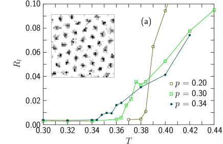
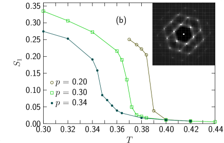
Figure 1: Collective pinning in the vortex solid. Panel (a) shows the linear resistance $R_{l}=\frac{1}{2}(R_{l,x}+R_{l,y})$ determined from Eq. (2) with $t=16384$ from data obtained with MC simulations. (The non-zero $R_{l}$ at low $T$ is an artifact of a rather small $t$ together with the fluctuations of $\Delta_{\mu}$ around a fixed values.) The inset is a top view of a configuration of vortices; the darker points indicates a higher density. Panel (b) shows the structure factor $S_{1}$; the inset is an intensity plot of $\ln S(\mathbf{k})$. Both insets are for $p=0.30$ and $T=0.30$. Note that the resistance, and thereby the mobility of the vortex solid, decreases rapidly as the temperature drops below melting.

Figure 2: Phase diagram for the simulated model. The open circles connected by a solid line is from determinations of melting temperatures from the vanishing of the structure factor; the continued dashed line is a sketch of a possible behavior at low temperatures. The “Floating solid” region at low $p$ is where the disorder strength is too weak to pin the vortex solid. This is a finite size effect; pinning is restored at a larger size. The filled circles show the location in the phase diagram of the runs in Fig. 3 at $T=0.24$ and the runs in Fig. 4 at $p=0.32$. The dashed region at low temperatures is where the numerical grid is expected to affect the results.

After having established the existence of collective pinning we turn to our main subject, which is the dynamics of a weakly driven system. At zero temperature the vortex lattice depins from the numerical grid at the critical current density $I_{0}\approx 0.13$, but our focus is on depinning from the disorder potential which takes place at current densities more than two orders of magnitude smaller than $I_{0}$. In the simulations the current is applied in the diagonal direction with $I_{x}=I_{y}=I/\sqrt{2}$ since this gives the force $f_{I}$ along $-\hat{\mathbf{v}}=(\hat{\mathbf{x}}-\hat{\mathbf{y}})/\sqrt{2}$ which is along one of the symmetry directions of the vortex lattice, see inset of Fig. 1(a). Likewise the voltage per link is $V=(V_{x}+V_{y})/\sqrt{2}$.

Figure 3 shows the $I$-$V$ characteristics at $T=0.24$ with four different pinning strengthssim . In the pure system, $p=0$, the voltage is proportional to the current, $V=R_{0}I$. The main effect of non-zero pinning strength is to shift the voltage down towards zero. As this shift downwards only depends weakly on $I$, the slope is almost independent of $p$. In this way we get a critical current density $I_{c}$ that separates the creep region with an unmeasurably low voltage at $I<I_{c}$ from the moving region at $I>I_{c}$ with $V\sim I-I_{c}$.

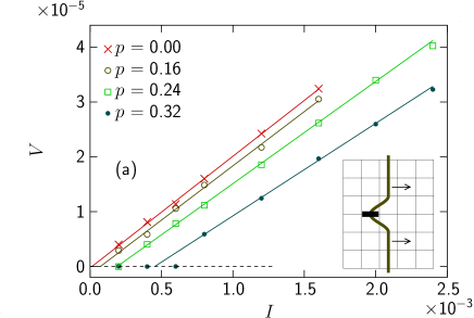
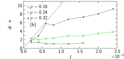
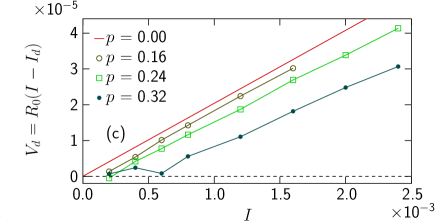
Figure 3: Results at $T=0.24$ and several different $p$. Panel (a) shows that the effect of a finite $p$ on the $I$-$V$ characteristics is to shift the data down towards zero. This gives a creep region with very low voltage at low currents, $I<I_{c}$, and a region with a rectilinear behavior at larger $I$. The inset which is a vortex line extending along $z$ and moving in the direction of the applied force, illustrates the suggested mechanism: the vortices at defect positions on the average lag after the moving vortex lattice. Panel (b) gives the displacement, c.f. Eq. (3) in the direction opposite to $f_{I}$. Panel (c) which is a calculation of the voltage from $R_{0}$ of the pure system and $I_{d}$ from the measured $d$ and Eq. (4), shows that the suggested mechanism captures the essential elements of the dynamics.

This behavior suggests the existence of a force which, much like a friction force, has to be overcome to set the vortices in motion and also reduces the velocity of the moving system. For a system in equilibrium one would expect the random pinning to contribute with a number of random forces which tend to cancel one another out, but the slow drift of the vortices opens up for other possibilities as e.g. memory effects. The idea behind our suggested mechanism is that some of the defect vortices initially stay fixed when the unpinned vortices slowly move in the direction of the force. This leads to distortions of the elastic vortex lines (see inset of Fig. 3(a)) and a gradual build-up of a force $f_{\mathrm{el}}$ on the defect vortices. This also gives a reaction force $f_{d}$ from the defect vortices on the vortex lattice; the motion of the vortex lattice should then be proportional to $f_{I}-f_{d}$.

A basic ingredient in this scenario is that the vortices at the defects on the average lag after the unpinned vortices. To test this idea we introduce a way to measure the average displacement of the defect vortices. To distinguish between ordinary vortices and defect vortices (or rather defect positions) we introduce the defect operator $D(\mathbf{r},z)$ which is unity at a defect and zero otherwise. The average position of all non-defect vortices belonging to the same vortex line may then be written,

$$\overline{\mathbf{r}}_{i}=\overline{[1-D(\mathbf{r}_{i}(z),z)]\;\mathbf{r}_{i}(z)},$$

and as a measure of the lagging behind of the defect vortices, we introduce the displacement as the sum of their deviations from the average vortex line positions,

$$\mathbf{d}=\left<\sum_{i,z}(\mathbf{r}_{i}(z)-\overline{\mathbf{r}}_{i})\;D(\mathbf{r}_{i}(z),z)\right>.$$ (3)

Note that this is only the displacements relative to the vortex lines. An estimate of a total displacement should also include effects due to a vortex line or a set of vortex lines lagging behind the rest of the vortex lattice. This is however considerably more difficult to estimate, and as we will see shortly it seems that the expression above contains the dominant contribution. Nevertheless, $\mathbf{d}$ is only an approximate estimate—most likely a lower bound—of the total displacement.

We now expect the displacement vector to be non-zero and point in the direction opposite to the force. Figure 3(b) which shows how $\mathbf{d}\cdot\hat{\mathbf{v}}$ depends on the applied current gives strong evidence for the suggested behavior; the defect vortices on the average lag after the ordinary vortices. For a qualitative comparison one would like to compare the magnitude of this defect force $f_{d}$ with $f_{I}$ from the applied current. We do a similar but more direct comparison by instead estimating $I_{d}$, the current in the system due to the displaced vortices. Recall that the creation of a vortex pair in a 2D model with a separation of $d$ lattice constants in the $y$ direction creates $d$ rows in the $x$ direction where the phase angle rotates by $2\pi$. This gives a total current $I_{\mathrm{tot}}\approx d\sin(2\pi/L_{x})\approx 2\pi d/L_{x}$. Taking this over to our 3D system we conclude that a displacement $d$ corresponds to a current density

$$I_{d}=\frac{I_{\mathrm{tot}}}{L_{y}L_{z}}\approx\frac{2\pi}{{\cal V}}d.$$ (4)

At $I<I_{c}$ we expect $I_{d}=I$ and it is then possible to obtain the displacement $d$ from Eq. (4). This is the dashed line in Fig. 3(b). The data for $I<I_{c}$ agrees well with this line. For the behavior at higher currents we plot in Fig. 3(c) $V_{d}=R_{0}(I-I_{d})$, which is an estimate of the voltage based on the measured displacement $d$, together with $R_{0}$ from the pure system. The agreement with Fig. 3(a) is good and shows convincingly that our simple description in terms of the displacement of the defect vortices captures the essential elements of the dynamics.

We now fix the pinning strength, $p=0.32$, and examine the $I$-$V$ characteristics at several different temperatures from $T=0.08$ to $T=0.30$. The results are shown in Fig. 4(a) and give evidence for a critical current that increases with decreasing temperature. In a further analysis we have found that it is possible to collapse the data by plotting the voltage versus the combination $TI$, see Fig. 4(b). This gives $I_{c}\propto 1/T$ and $V(T,I)=\chi(I/I_{c})$ where $\chi$ is a scaling function. To check if this behavior is general or depends crucially on our way of introducing the disorder as a low density of very strong defects, we have done additional simulations with random couplings as in Ref. Olsson and Teitel, 2001 with $p=0.08$. These simulations give support for the same kind of scaling collapse.

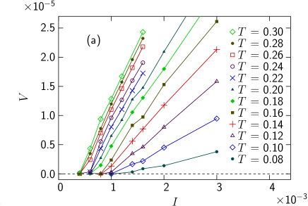
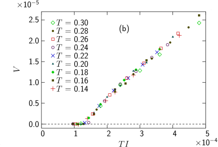
Figure 4: The voltage at $p=0.32$ and several different temperatures. Panel (a) gives evidence for a critical current that increasese with decreasing temperature. Panel (b) shows that the voltage may be collapsed to an impressing accuracy by plotting the data versus $TI$.

At low temperatures one expects an effect of the discrete lattice would be to slow down the dynamics. This is precisely what is seen at $T\leq 0.12$ (the data fall below the common curve) and this data is therefore discarded to produce the collapse in Fig. 4(b). To study the effect of the discretization we return to the behavior of the linear resistance in a clean system. At high temperatures the linear resistance decreases slowly with temperature down to $T\approx 0.22$ where it starts falling rather rapidly down to $R_{l}=0$ at $T=0.14$. This shows that the effects of the discrete grid are significant up to $T\approx 0.22$. Since the discretization is expected to be unimportant if the typical wandering of the vortex line is much larger than the lattice spacing, we examine the mean-squared fluctuation which is $\left<u^{2}\right>=1.03$ at $T=0.22$. It also turns out that the data at low $T$ that were discarded in Fig. 4(b) all have $\left<u^{2}\right><1$ whereas $\left<u^{2}\right>>1$ at the temperatures included in the figure. This suggests $\left<u^{2}\right>\gtrsim 1$ as a criterion for significant effects due to the discretization (the dashed region in Fig. 2), and gives support to our claim that the failure to collapse the data at low $T$ actually is an effect of the discretization of the underlying grid.

The origin of the collapse in Fig. 4(b) is surprising as several quantities that could be expected to affect the mobility change considerably across this temperature interval. Examples are the fraction of vortices on defect positions that decreases from 0.078 at $T=0.14$ to 0.054 at $T=0.30$, the structure factor that decreases from 0.5 to 0.3, and the resistance in the absence of disorder which behaves as $R_{0}(T)\sim T^{1/2}$.

To conclude, we have obtained the $I$-$V$ characteristics of a point disordered frustrated 3D XY model and found that the effect of disorder is to give a critical current that separates the creep region from a region with $V\sim I-I_{c}$. The reason for this behavior is a pinning force which appears to be due to a memory effect; a fraction of the defect vortices lag after the rest of the vortex lattice. Finally, it is shown that the voltage may be collapsed by plotting the voltage versus $TI$, though the origin of this behavior as yet not is fully understood.

We acknowledge discussions with S. Teitel and P. Minnhagen, support by the Swedish Research Council contract No. 2002-3975, and access to the resources of the Swedish High Performance Computing Center North (HPC2N).

References

- Nattermann (1990) T. Nattermann, Phys. Rev. Lett. 64, 2454 (1990).
- Giamarchi and Doussal (1994) T. Giamarchi and P. Le Doussal, Phys. Rev. Lett. 72, 1530 (1994).
- Beidenkopf et al. (2005) H. Beidenkopf, N. Avraham, Y. Myasoedov, H. Shtrikman, E. Zeldov, B. Rosenstein, E. H. Brandt, and T. Tamegai, Phys. Rev. Lett. 95, 257004 (2005).
- Li and Rosenstein (2003) D. Li and B. Rosenstein, Phys. Rev. Lett. 90, 167004 (2003).
- Hernández and Domínguez (2004) A. D. Hernández and D. Domínguez, Phys. Rev. Lett. 92, 117002 (2004).
- Olsson (1994) P. Olsson, Phys. Rev. Lett. 73, 3339 (1994).
- Nonomura and Hu (2001) Y. Nonomura and X. Hu, Phys. Rev. Lett. 86, 5140 (2001).
- Kim et al. (1999) B. J. Kim, P. Minnhagen, and P. Olsson, Phys. Rev. B 59, 11506 (1999).
- Chen and Hu (2003) Q.-H. Chen and X. Hu, Phys. Rev. Lett. 90, 117005 (2003).
- (10) If the voltage is plotted on a log scale it becomes clear that it is very similar to corresponding data in Fig. 2(a) in Ref. Hernández and Domínguez, 2004.
- Olsson and Teitel (2001) P. Olsson and S. Teitel, Phys. Rev. Lett. 87, 137001 (2001).