Asymmetric Fermi superfluid in a harmonic trap

Abstract

We consider a dilute two-component atomic fermion gas with unequal populations in a harmonic trap potential using the mean field theory and the local density approximation. We show that the system is phase separated into concentric shells with the superfluid in the core surrounded by the normal fermion gas in both the weak-coupling BCS side and near the Feshbach resonance. In the strong-coupling BEC side, the composite bosons and left-over fermions can be mixed. We calculate the cloud radii and compare axial density profiles systemically for the BCS, near resonance and BEC regimes.

1 Introduction:

The original BCS state for superconductors considers pairing between two species of fermions with equal populations. For a long time, theorists studied the fermion system with unequal species, or mismatched Fermi surfaces, and proposed this system may have different ground state [1], in particular the so called Fulde-Ferrell-Larkin-Ovchinnikov (FFLO) phase. Experimentally, however, such superfluid states remain unclear because of the difficulty in preparing the magnetized superconductors.

Experiments with ultra-cold atoms have opened a new era to study this fermion system with unequal populations. Through the Feshbach resonance [2], the effective interaction between atoms can be varied over a wide range such that the ground state can be turned from a weak-coupling BCS superfluid to a strong-coupling Bose-Einstein condensation (BEC) regime. In the homogeneous system, theoretical studies [3, 4, 5] of the unequal fermion species show that the phase transition must occur when the resonance is crossed, in contrast to the equal population case where a smooth crossover takes place [6, 7]. Breached pair phase [8], phase separated states are also proposed [9, 10] in this system.

Two recent experiments [11, 12] studied the trapped ⁶Li atoms with imbalanced spin populations and obtained the density profiles for various population differences. Both groups found the system contains a superfluid core surrounded by a normal fermions and provide evidence for phase separation near the crossover.

In this paper, we study this imbalanced fermion system by mean field approximation and evaluate the density profiles for various coupling strengths from weak-coupling BCS superfluid to strong coupling BEC regime. In particular, we calculate the axial density profiles, superfluid and minority cloud radii, and distinguish between the phase separation and Bose-Fermi mixture regimes. This paper is organized as follows: In Sec. II we briefly review the mean-field approximation for the dilute fermion atoms with unequal populations. In Sec. III we present our results for various polarizations from weaking-coupling BCS superfluid to strong-coupling BEC side. We show that the axial density profiles are constant within the superfluid core and decrease beyond the phase boundary for the phase separations but are smoothly decreasing functions for entire trap for the mixtures. Finally, we conclude with a briefly summary in Sec. IV.

While this work was in progress, several theoretical papers have also studied the same problem under similar approximations [13, 14, 15, 16] or going beyond [17, 18]. Basically, ref [13, 14, 15, 16, 17] also conclude the system is phase separated into concentric shells with superfluid in the center and surrounding by leftover fermions near the resonance. The strong-coupling BEC limit has also been studied [13, 14, 18]. In this case, the composite bosons and unpaired fermions can mix. As the population difference increases the unpaired fermions can even penetrate into the superfluid core. Our paper provides a more systematic study of the entire BCS-BEC regimes for all polarizations.

2 Formalism:

Restricting ourselves to wide Feshbach resonance, the two-component fermion system can be described by an effective one-channel Hamiltonian

$$H\ =\ \sum_{{\bf k},\sigma}\xi_{\sigma}({\bf k})c^{\dagger}_{{\bf k},\sigma}c_{{\bf k},\sigma}\ +\ g\sum_{\bf k,k^{\prime},q}c^{\dagger}_{{\bf k+q},\uparrow}c^{\dagger}_{{\bf k^{\prime}-q},\downarrow}c_{{\bf k^{\prime}},\downarrow}c_{{\bf k},\uparrow}\ ,$$ (1)

where $\xi_{\sigma}({\bf k})\,=\,\hbar^{2}k^{2}/2m-\mu_{\sigma}$ and the index $\sigma$ runs over the two spin components. Within the BCS mean field approximation at zero temperature, the excitation spectrum in a homogeneous system for each spin is (see e.g. [20] for details)

$$E_{\sigma}({\bf k})\,=\,\frac{\xi_{\sigma}({\bf k})-\xi_{-\sigma}({\bf k})}{2}\ +\ \sqrt{\left(\frac{\xi_{\sigma}({\bf k})+\xi_{-\sigma}({\bf k})}{2}\right)^{2}\,+\,\Delta^{2}}\ ,$$ (2)

where $\xi_{\sigma}({\bf k})\,=\,\hbar^{2}k^{2}/2m-\mu_{\sigma}$ are the quasi-particle excitation energies for normal fermions, and $-\uparrow\equiv\downarrow$. For an inhomogeneous system, $e.g.$ the system in a harmonic trap, a finite system sized effect should be included [19]. However, the system can be treated as homogeneous locally if the number of particles are sufficiently large. A local density approximation, or Thomas-Fermi approximation (TFA), is applied and the chemical potential for spin $\sigma$ is replaced by

$$\mu_{\sigma}(r)\ =\ \mu^{0}_{\sigma}\ -\frac{1}{2}m\omega^{2}r^{2}\ ,$$ (3)

with $\omega$ the isotropic trap frequency and $r$ the distance from the trap center. We shall show results explicitly only for the isotropic trap. In the local density approximation, the densities $n_{\sigma}({\bf r})$ depends only on the local chemical potentials $\mu_{\sigma}({\bf r})$. Hence the density profile of an anisotropic trap can be related to an isotropic one by rescaling the spatial coordinates appropriately. We then introduce the average chemical potential

$$\mu(r)\ \equiv\ \frac{1}{2}[\mu_{\uparrow}(r)+\mu_{\downarrow}(r)]\ =\ \mu_{0}\ -\ \frac{1}{2}m\omega^{2}r^{2}\ ,$$ (4)

and the difference $h\ \equiv\ [\mu_{\uparrow}(r)-\mu_{\downarrow}(r)]/2\,=\,(\mu^{0}_{\uparrow}-\mu^{0}_{\downarrow})/2$. The dispersion relation in Eq. (2) becomes

$$E_{\uparrow,\downarrow}({\bf k,r})\,=\,\sqrt{\xi({\bf k,r})^{2}+\Delta^{2}({\bf r})}\mp h$$ (5)

where $\xi({\bf k,r})\equiv\hbar^{2}k^{2}/2m-\mu(r)$. We take spin up to be the majority species so that $h$ and $E_{\uparrow}$ are positive always. Then the density profiles in a harmonic trap are

$$n_{s}(r) = n_{\uparrow}(r)+n_{\downarrow}(r)\ =\ \int{d^{3}k\over(2\pi)^{3}}\left[1-{2\xi({\bf k,r})\over E_{\uparrow}+E_{\downarrow}}f(-E_{\uparrow})\right]\ ,$$ (6)

$$n_{d}(r) = n_{\uparrow}(r)-n_{\downarrow}(r)\ =\ \int{d^{3}k\over(2\pi)^{3}}f(E_{\uparrow})\ ,$$ (7)

and the total number of particles $N\,=\,\int d^{3}rn_{s}(r)$. Here $f$ is the Fermi function. The polarization of the system is defined as

$$P\ \equiv\ {N_{\uparrow}-N_{\downarrow}\over N}\ =\ {1\over N}\int d^{3}rn_{d}(r)\ .$$ (8)

Now the pairing field $\Delta$ depends on position also. In the local density approximation, it obeys an equation similar to the homogeneous case [4, 20]:

$$-\frac{m}{4\pi a}\Delta(r)\,=\,\Delta(r)\int\frac{d^{3}k}{(2\pi)^{3}}\left[\frac{1-f(E_{\uparrow})-f(E_{\downarrow})}{E_{\uparrow}+E_{\downarrow}}\,-\,\frac{m}{\hbar^{2}k^{2}}\right]\ .$$ (9)

For a given scattering length $a$, we solve equations (6), (7) and (9) self-consistently for fixed total number of particles $N$ and polarization $P$. The solutions to the“gap equation” (9) may not be unique. The physical solution is determined by the condition of minimum free energy among the multiple solutions. We describe the detail procedures in A.

3 Results and Discussions

In this section, we investigate the density profiles for various polarizations and coupling strengths from positive detuning BCS superfluid to negative detuning BEC side. With the aid of density profiles, we evaluate the radii of the superfluid phase boundaries for various cases and compare to the current experimental results. We close this section with a discussion of axial density profiles. Phase separation versus Bose-Fermi mixture can be clarified through the axial density profiles of the population difference.

In Fig. 1, we plot the radial density profiles for three different coupling strengths $1/k_{F}a\,=\,-0.61,\,0.03$, and $2.44$ (for different columns) with polarization $P\,=\,0.2\,,0.5$, and $0.9$ (for different rows). The total number of particles are fixed to $2\times 10^{5}$. Here $k_{F}$ is the Fermi wavevector at the trap center for an ideal symmetric Fermi gas with the same total number of particles. In all these plots, the system shows a superfluid cloud surrounded by a normal Fermi gas except the case in Fig. 1(c) where the system is completely in the normal state with the polarization $P=0.9$. It is consistent with the experimental observation [11] that the superfluid is destroyed by a sufficiently large population difference. We remark here however that the critical population difference $P_{c}$ for the destruction of superfluidity obtained here is much larger than that found in the experiment [11]. For $1/k_{F}a=-0.61$ here, $P_{c}>0.6$ theoretically whereas an extrapolation of the data of [11] gives $P_{c}<0.3$ (see further discussions below). For less polarized system on the BCS side [Fig. 1(a) and (b)], it shows a clear phase separation between the superfluid and a normal Fermi gas. Note that within the superfluid cloud, the population difference is zero and the system is just like the typically unpolarized superfluid. Outside the superfluid cloud, both components of the fermions exist in the normal state which indicates a fraction of the fermions which are not paired-up even at the zero temperature. The density profile of the population difference $n_{d}(r)$ peaks at the superfluid phase boundary and decreases gradually toward the edge of the trap. Its value is equal to the density profile of the majority when $r\geq r_{\downarrow}$, the radii of the minority cloud. At the superfluid phase boundary, both the majority and minority density profiles exhibit discontinuous which has been observed also by the others [13, 14, 15].

Near resonance [Fig. 1(d)-(f)], similar phase separated states are observed. However, most of the minority are paired up in this regime such that the density profiles contains mainly the excess fermions outside the superfluid cloud at all $P$’s. This is consistent with the homogeneous normal phase boundary extends near resonance to large population difference [4]. Near resonance, the superfluid core survives at $P=0.9$ in our calculations whereas experimentally [11] it vanishes already at $P\approx 0.7$.

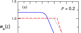
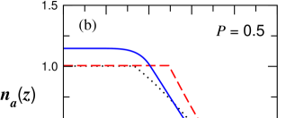
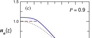
Figure 4: (color online). Axial population density difference $n_{a}(z)$ versus $z/R_{TF}$. $R_{TF}$ is defined in the caption of Fig 1. $n_{a}(z)$ is normalized to $1$ at $z=r_{s}$.

On the BEC side [Fig. 1(g)-(i)], all of the minority are paired up and the excess fermions can penetrate into the superfluid core. The system contains a superfluid core for any $P$ (if sufficiently deep in the BEC regime, see Fig. 4 below). The system then contains three different phases: the purely superfluid, the mixture phase, and the normal fermions from the trap center to the edge of the trap. The mixture phase extends toward the trap center as the polarization increases. In Fig. 1(i) ($P=0.9$), the system is highly polarized and the excess fermions extend deeply into the trap center. In B, we give an analytic discussion of the density profiles in the BEC limit.

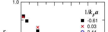
Figure 2: (color online). Radii of the superfluid core $r_{s}$ versus polarization $P$ for normalized coupling strengths in the legend.

The radius $r_{s}$ of the superfluid core is one of the most interesting quantities in current studies of the imbalanced fermion system [12, 14, 15, 16, 17]. From Fig. 1, the density profiles of the population difference $n_{d}(r)$ have maxima at the phase boundaries between the superfluid and the normal fermions. $r_{s}$ is thus also the peak position of $n_{d}(r)$. In Fig. 2, we plot $r_{s}$ as function of $P$ for three different coupling strengths. $r_{s}$ behaves quite differently above and below the resonance. On the BCS side the superfluid is eliminated when the polarization reaches around 0.65 for $1/(k_{F}a)=-0.61$ and the system becomes completely normal with mismatch Fermi surfaces beyond this critical polarization. For large coupling strengths, $r_{s}$ is finite except when $P$ is exactly $1$, since the superfluid is stable for any finite ($\neq 1$) polarization in the homogeneous case [4]. Except for small ($P\leq 0.1$) or large ($P\geq 0.9$) polarizations, the sizes of the superfluid clouds have maxima near the Feshbach resonance at fixed polarization.

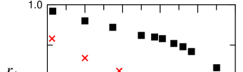
Figure 3: (color online). Radii of the minority species $r_{\downarrow}$ versus polarization $P$ for normalized coupling strengths in the legend.

We also plot the radii ($r_{\downarrow}$) of the minority (spin down fermions) cloud in Fig. 3. Below the Feshbach resonance, this radius is the same as the radius of the superfluid core because all the minority of fermions are paired up. However, this won’t be true above the Feshbach resonance where part of minority are not paired up in this regime. Unlike $r_{s}$, $r_{\downarrow}$ decreases monotonically as the coupling strength increases. These two radii become identical when the minority are paired up completely when the system reaches the BEC regime.

Due to the experimental constraints, one can not measure the radial density profiles directly. Instead the axial density profiles are reported in [12]. In Fig. 4, we plot the normalized axial density profiles $n_{a}(z)$ $[\equiv\int dxdyn_{d}(\vec{r})]$ of the population difference for different coupling strengths at three fixed polarization $P$. For the cases with phase separations [Figs. 1(a), (b), and (d)-(f)] , the corresponding $n_{a}(z)$ are constants for $z\leq r_{s}$ and have a kink at the phase boundary (for $z=r_{s}$). This feature results from the population difference $n_{d}(r)$ being zero inside the superfluid cloud (see C in detail) such that $n_{a}(z)$ remains the same value as at the phase boundary $z=r_{s}$. For a system with a mixed phase region [Figs. 1(g)-(i)], $n_{a}(z)$ increases smoothly toward the trap center even as $z\leq r_{s}$. It reaches a constant value within the cloud containing superfluid only [ $e.g.$, the cases with solid lines in Figs. 4(a) and (b)]. At large polarization [solid line in Fig. 4(c)], the excess fermions mix with superfluid entirely for $1/k_{F}a\,=\,2.44$ such that $n_{a}(z)$ increases monotonically toward the trap center. The completely different features for the axial density profiles of the population difference inside the superfluid cloud can help us to clarify whether the system is phase separation or mixture.

4 Conclusion

We have investigated the radial density profiles of the two-component fermion system with unequal spin-populations under Feshbach resonance. The system shows a superfluid cloud in the trap center surrounding by normal fermions. In the weak-coupling BCS side, the superfluid is destroyed completely at the polarization $P\,\gtrsim\,0.65$ for $1/(k_{F}a)=-0.61$. Near the Feshbach resonance, almost all the minority are paired up and the system is phase separated into superfluid and the normal fermions. In the strong-coupling BEC side, the excess fermions can mix with the superfluid and the system contains three different phases, the purely superfluid cloud, the mixture phase, and the normal fermions from the trap center to the edge of the trap.

In particular, we emphasize the difference in the axial density difference profiles between the phase separation and Bose-Fermi mixture regimes. The former shows a constant for $z<r_{s}$ and has a kink at the phase boundary but the later are smoothly increasing toward the trap center. However, Ref. [12] reported positive slopes of the axial density different profiles inside the superfluid cloud that indicates the $n_{d}(\vec{r})$ need to be negative somewhere within the superfluid cloud. We do not obtain this phenomenon within current local density approach.

Appendix A Free energy

To determine the minimum free energy state when there are multiple solutions, we need an expression for the free energy. We obtain this as follows. First consider a system with fixed volume $V$ and particle numbers $N_{\sigma}$. With the Hamiltonian in Eq. (1), it is straight-forward to show that [21] the energy $E(N_{\sigma},g)$ of this system obeys

$$\frac{\partial E}{\partial g}=\frac{V}{g^{2}}|\Delta|^{2}\ .$$ (10)

We need to eliminate $g$ in favor of the scattering length $a$, the physical parameter of the system. These two variables are related by the expression

$$\frac{m}{4\pi\hbar^{2}a}\ =\ \frac{1}{g}+\frac{1}{V}\sum_{\vec{k}}\frac{1}{2\epsilon_{k}}\ .$$ (11)

We thus get

$$\frac{m}{4\pi\hbar^{2}}d\left(\frac{1}{a}\right)=d\left(\frac{1}{g}\right)\ ,$$ (12)

and therefore

$$\frac{\partial E}{\partial(1/a)}|_{N_{\sigma}}=-V\frac{m}{4\pi\hbar^{2}}|\Delta(a)|^{2}\ .$$ (13)

Writing this derivative to be ${\cal E}^{\prime}$, we then get the thermodynamic relation

$$dE=\sum_{\sigma}\mu_{\sigma}dN_{\sigma}+{\cal E}^{\prime}d(\frac{1}{a})\ .$$ (14)

The free energy $\Omega(\mu_{\sigma},a)\equiv E-\mu_{\uparrow}N_{\uparrow}-\mu_{\downarrow}N_{\downarrow}$ then obeys

$$d\Omega=-\sum_{\sigma}N_{\sigma}d\mu_{\sigma}+{\cal E}^{\prime}d(\frac{1}{a})\ .$$ (15)

We thus conclude that, for volume $V$ and chemical potentials $\mu_{\sigma}$,

$$\frac{\partial\Omega}{\partial(1/a)}|_{\mu_{\sigma}}=-V\frac{m}{4\pi\hbar^{2}}|\Delta|^{2}\ .$$ (16)

Though this expression is already sufficient to determine and thus compare the free energies of the different solutions for given scattering length $a$, we can convert it to an even more convenient form. To do this, let us write $x\equiv|\Delta|^{2}$ and $y\equiv 1/a$. We get, up to an overall multiplying factor

$$\frac{\partial\Omega}{\partial y}=-x\ .$$ (17)

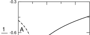
Figure 5: Solution to the gap equation plotted as $1/a$ vs $|\Delta|^{2}$ (arbitrary units) for the case with multiple solutions (dashed lines). The minimum energy solution is shown as the thick black line. The areas labeled by A and B are equal.

Thus, when the solutions are plotted in the form of Fig. 5, the free energy $\Omega$ of a state can be related to the free energy $\Omega_{0}$ of another state along the same curve by, again up to an overall multiplicative constant,

$$\Omega=\Omega_{0}-\int xdy\ .$$ (18)

Since $\int xdy$ is the area between the curve and the y-axis, the states corresponding to the minimum free energy at a given scattering length $a$ (hence $y$) can be found via the same procedure as the usual Maxwell construction.

Appendix B BEC limit

Here we try to understand the behaviour of the density profile in the BEC ($1/k_{F}a\gg 1$) limit, for the special case of small number of excess fermions [$e.g.$ Fig. 1(g)]. For a bulk system, it is straight forward to perform a low density expansion of the mean-field equations and obtain an expansion of the chemical potentials $\mu_{f}\equiv\mu_{\uparrow}$ and $\mu_{b}\equiv\mu_{\uparrow}+\mu_{\downarrow}$ as a series in the densities $n_{f}=n_{d}$ and $n_{b}\equiv n_{\downarrow}$ (see [22] for the details of this calculation). In the BEC limit, $n_{d}$ can be interpreted as the density of the excess unpaired fermions and $n_{b}$ as the density of the bosons which represent the bound fermion pairs. $\mu_{f}$ and $\mu_{b}$ can be interpreted as the corresponding chemical potentials. Explicitly we have an expansion of the form

$$\mu_{f} = An_{d}^{2/3}+g_{bf}n_{b}\ ,$$ (19)

$$\mu_{b} = -\epsilon_{b}+g_{bb}n_{b}+g_{bf}n_{f}\ ,$$ (20)

where we have dropped the terms higher order in the densities. These terms are smaller in the limit $n_{f}a^{3}\ll 1$ and $n_{b}a^{3}\ll 1$. We obtain [22] $A=(6\pi^{2})^{2/3}/2m$, $\epsilon_{b}=\hbar^{2}/ma^{2}$, $g_{bb}=4\pi\hbar^{2}a/m$, $g_{bf}=8\pi\hbar^{2}a/m$. The value of $A$ is as expected for a free Fermi gas and $\epsilon_{b}$ is the binding energy of the fermion pair. The values of $g_{bb}$ and $g_{bf}$ here, obtained from the mean-field equations, differ from the correct values known. Exact three-body calculation [23] gives $g_{bf}^{\rm exact}=3.6\pi\hbar^{2}a/m$, while a recent four-body calculation [24] gives $g_{bb}^{\rm exact}=1.2\pi\hbar^{2}a/m$. Alternatively, defining the scattering lengths in the usual manner, our low density expansion yields the effective values $a_{bf}=8a/3$ and $a_{bb}=2a$, whereas the exact values should be $a_{bf}^{\rm exact}=1.2a$ and $a_{bb}^{\rm exact}=0.6a$. The difference between the mean-field and exact results is due of course to the approximate nature of the mean-field theory. We note however, here that (a) $a_{bf}$ and $a_{bb}$ are both positive and of order $a$, hence in the BEC limit we have necessarily $n_{d}a^{3}\ll 1$, thus the fermions and the bosons can mix [25]; (b) $g_{bf}/g_{bb}>1/2$ for both mean-field and exact values. We shall explain the importance of this second relation below.

In the trap, Eqs. (19) and (20) becomes

$$\mu_{f} = An_{d}(\vec{r})^{2/3}+g_{bf}n_{b}(\vec{r})+V(\vec{r})\ ,$$ (21)

$$\mu_{b} = -\epsilon_{b}+g_{bb}n_{b}(\vec{r})+g_{bf}n_{f}(\vec{r})+2V(\vec{r})\ .$$ (22)

Here $V(\vec{r})$ is the trap potential. We shall only consider the case where the potential increases from the center of the trap. To appreciate the implications of the relation (b), consider the limit of a small number of fermions. The density profile of the bosons can then be determined by first ignoring the fermion term in Eq. (21), and we obtain the boson density profile

$$n_{b}(\vec{r})=(\mu_{b}+\epsilon_{b}-2V(\vec{r}))/g_{bb}\ ,$$ (23)

if the R.H.S. is larger than zero, and $n_{b}=0$ otherwise. For ease of reference, we shall call these two regions “inside” and “outside” below.

Eq. (21) can be rewritten in the form

$$\mu_{f}=An_{d}(\vec{r})^{2/3}+V_{\rm eff}(\vec{r})\ ,$$ (24)

where $V_{\rm eff}(\vec{r})=V(\vec{r})+g_{bf}n_{b}(\vec{r})$ is the effective potential for the fermions. We obtain, for the inside region, $V_{\rm eff}(\vec{r})=V(\vec{r})+(g_{bf}/g_{bb})(\mu_{b}+\epsilon_{b}-2V(\vec{r}))$ whereas for the outside $V_{\rm eff}(\vec{r})=V(\vec{r})$. In the inside region, the position dependence is therefore $-(2g_{bf}/g_{bb}-1)V(\vec{r})$. From this, it is clear that if $g_{bf}>g_{bb}/2$, then the effective potential actually is larger near $\vec{r}=0$ than near the edge of the boson cloud. It decreases from the center of the trap till it reaches the edge of the boson cloud, then it increases again due to the spatial dependence of $V(\vec{r})$. Therefore, we conclude that for ${g_{bf}}/{g_{bb}}>1/2$, the excess fermions lie near the edge of the boson cloud, at least for a small number of Fermions [26, 18]. The excess fermions lie near the edge of the cloud [Fig. 1(g)]. Thus a peak in $n_{d}(\vec{r})$ does not indicate phase separation.

Appendix C Axial Density

We here discuss some useful expressions governing the axial density within the local density approximation. Our results here are, to some extent, a further development of those obtained in [14].

In local density approximation, any quantity, say the density difference $n_{d}(\vec{r})$, is a function entirely of the local chemical potential $\mu(\vec{r})$ (note that $h$ is a constant). Hence, we can write

$$n_{d}(\vec{r})=g(\mu(\vec{r}))\equiv g(\mu(\vec{r}),h)$$ (25)

for some function $g$. We here note that any density must be identically zero for sufficiently large and negative chemical potential, and thus $g(\zeta)$ vanishes exactly for sufficiently large and negative argument $\zeta$. It will be convenient to define another function $G(\zeta)$ via

$$G(\zeta)\equiv\int_{-\infty}^{\zeta}d\zeta^{\prime}g(\zeta^{\prime})\ .$$ (26)

Consider now for example the radially integrated density (referred afterwards as axial density) difference:

$$n_{a}(z)\equiv\int dxdyn_{d}(\vec{r})\ .$$ (27)

The integral can be written as, for a trap that is cylindrically symmetric with respect to $z$, $\pi\int_{0}^{\infty}d\rho^{2}g(\mu_{0}-\frac{1}{2}\alpha_{z}z^{2}-\frac{1}{2}\alpha_{\parallel}\rho^{2})$ where $\rho^{2}\equiv x^{2}+y^{2}$. This integral can be expressed in terms of $G$ and thus

$$n_{a}(z)=\frac{2\pi}{\alpha_{\parallel}}G(\mu_{0}-\frac{1}{2}\alpha_{z}z^{2})\ .$$ (28)

This relation can be used to obtain directly the axial density in terms of the function $g$, without first calculating the density profile in trap and then performing the integration. Moreover, it can also be used to deduce the (unintegrated) density profile once the axial density is given, for example from experiment. To see this, we differentiate Eq. (28) with respect to $z$, and notice that $G^{\prime}(\zeta)=g(\zeta)$ evaluated at $\zeta=\mu_{0}-\frac{1}{2}\alpha_{z}z^{2}$ is directly related to the corresponding density at the coordinate $(0,0,z)$. Thus we have

$$n_{d}(0,0,z)=-\frac{\alpha_{\parallel}}{2\pi\alpha_{z}}\frac{1}{z}\frac{\partial n_{a}(z)}{\partial z}\ .$$ (29)

Therefore the actual density for a point on the $z$ axis can be obtained from the axial density. Under the local density approximation, the density at any given point in the trap is a function of the local chemical potential only. Hence we can obtain the actual density at any given point in space provided the axial density is given.

The relation Eq. (29) also shows that, since $n_{d}$ is non-negative, the axial density profile is strictly decreasing (increasing) with $z$ for $z\,>\,(<)\,0$, a result pointed out in reference [14]. In a region where the density vanishes, then the axial density should be a constant, a result recognized in references [14] and [15].

References

Figure 1: (color online). Radial density profiles for $n_{\uparrow}(r)$ (solid lines), $n_{\downarrow}(r)$ (dashed lines), and $n_{d}(r)$ (solid circles). The dotted lines are the normal state density profile with the same density as in the normal region. The coupling strengths (each column) $1/(k_{F}a)=$ -0.61 (left, BCS-side), 0.03 (middle, near resonance), 2.44 (right, BEC-side) and the polarizations (each row) $P=$ 0.2, 0.5, and 0.9. The total number of fermions are fixed to $N=2.0\times 10^{5}$. $R_{TF}$ is the size of the Thomas-Fermi radius of the normal spin-up cloud.

References

- [1] Fulde P and Ferrell R A 1964 Phys. Rev.135 A550 Larkin A I and Ovchinnikov Y N 1964 Zh. Éksp. Teor. Fiz. 47 1136 [1965 Sov. Phys.–JETP 20 762]
- [2] Tiesinga E, Verhaar B J and Stoof H T C 1993 Phys. Rev.A 47 4114 Inouye S, Andrews M R, Stenger J, Miesner H-J, Stamper-Kurn D M and Ketterle W 1998 Nature 392 151 Courteille P, Freeland R S, Heinzen D J, van Abeelen F A and Verhaar B J 1998 Phys. Rev. Lett.81 69 Roberts J L, Claussen N R, Burke J P Jr., Greene C H, Cornell E A and Wieman C E 1998 Phys. Rev. Lett.81 5109
- [3] Carlson J and Reddy S 2005 Phys. Rev. Lett.95 060401
- [4] Pao C-H, Wu S-T and Yip S-K 2006 Phys. Rev.B (to be published)
- [5] Sheehy D E and Radzihovsky L 2006 Phys. Rev. Lett.96 060401 Son D T and Stephanov M A 2005 Preprint cond-mat/0507586
- [6] Eagles D M 1969 Phys. Rev.186 456 Leggett A L 1980 Modern Trends in the theory of condensed matter ed Pekalski A and Przystawa J (Springer-Verlag: Berlin)
- [7] Sá de Melo C A R, Randeria M, and Engelbrecht J R 1993 Phys. Rev. Lett.71 3202
- [8] Forbes M M, Gubankova E, Liu W V and Wilczek F 2005 Phys. Rev. Lett.94 017001 and references therein
- [9] Bedaque P F, Caldas H and Rupak G 2003 Phys. Rev. Lett.91 247002
- [10] Caldas H 2004 Phys. Rev.A69, 063602
- [11] Zwierlein M W, Schirotzek A, Schunck C H and Ketterle W 2006 Science 311 492
- [12] Partridge G B, Li W, Kamar R I, Liao Y and Hulet R G 2006 Science 311 503
- [13] Yi W and Duan L-M 2006 Preprint cond-mat/0601006
- [14] De Silva T N and Mueller E J 2006 Preprint cond-mat/0601314
- [15] Haque M and Stoof H T C 2006 Preprint cond-mat/0601321
- [16] Chevy F 2006 Preprint cond-mat/0601122
- [17] Kinnunen J, Jensen L M and Törmä P 2005 Preprint cond-mat/0512556
- [18] Pieri P and Strinati G C 2005 Preprint cond-mat/0512354
- [19] Bruun G, Castin Y, Dum R and Burnett K 1999 Eur. J. Phys.D 7 433
- [20] Wu S-T and Yip S-K 2003 Phys. Rev.A 67 053603
- [21] Abrikosov A A, Gorkov L P and Dzyaloshinskii I E, 1965 Quantum Field Theoretical Methods in Statistical Physics (Pergamon: Oxford) Lifshitz E Mand Pitaevskii L P 1980 Statistical Physics Part 2 (Pergamon: Oxford) Chapter 5 sec 40. Note however that our sign convention for is opposite to these references.
- [22] Yip S K 2002 Preprint cond-mat/0203582
- [23] Skorniakov G V and Ter-Martirosian K A 1956 Zh. Th. Eksp. Theo. 31 775 [Sov. Phys.–JETP 4 648]
- [24] Petrov D, Salomon C and Shlyapnikov G V 2004 Phys. Rev. Lett.91, 090404
- [25] Viverit L, Pethick C J and Smith H 2000 Phys. Rev.A 41 053605
- [26] Carr L D, Chiaramonte R and Holland M J 2004 Phys. Rev.A70, 043609