Decoherence and dephasing in Kondo tunneling through double quantum dots

Abstract

We describe the mechanism of charge-spin transformation in a double quantum dot (DQD) with even occupation, where a time dependent gate voltage $v_{g}(t)$ is applied to one of its two valleys, whereas the other one is coupled to the source and drain electrodes. The Kondo tunneling regime under strong Coulomb blockade may be realized when the spin spectrum of the DQD is formed by the ground state spin triplet and two singlet excitations. Charge fluctuations induced by $v_{g}(t)$ result in transitions within the spin multiplet characterized by the $SO(5)$ dynamical symmetry group. In a weakly non-adiabatic regime the decoherence, dephasing and relaxation processes affect Kondo tunneling. Each of these processes is caused by a special type of dynamical gauge fluctuations, so that one may discriminate between the decoherence in the ground state of a DQD and dephasing at finite temperatures.

I Introduction

Manipulating spins in quantum dots in order to achieve new ways of processing information has been a subject of intense research in the last decade. qucom One of the basic building blocks for quantum computing is a double quantum dot (DQD),dqd where the concepts of entanglement and phase accumulation may be effectively modelled and studied. entangl It turns out that the key problem, which hampers the progress in implementing the quantum information storage and processing is the impossibility of perfect isolation of a complex quantum system from the environment, which results in the loss of quantum coherence.deco The phase coherence of tunnel transport through a quantum dot can be effectively controlled in an Aharonov-Bohm geometry abohm and/or in the Kondo regime.kondr To understand the generic features of the decoherence phenomenon, various model situations are considered, where dephasing and relaxation processes are controlled by specific mechanisms of interaction with the external environment. Among these processes the interaction with a phonon bath gurv and an electron liquid KNG ; Paas should be regarded as typical examples.

The aim of this paper is to study a specific mechanism of decoherence and dephasing, which stems from the violation of dynamical symmetry in a DQD. This dynamical symmetry is an intrinsic property of any quantum dot with even occupation, where the low-energy spectrum of spin excitations is formed by singlet (S) and triplet (T) states. KA01 ; Nova Since the interaction with a reservoir (electrons in metallic leads) violates the spin conservation law, S/T transitions accompany the cotunneling through DQD and thus contribute to the tunneling transparency and, in particular, to the Kondo-type zero-bias anomaly in tunnel conductance.

The physical system in which we will study decoherence and dephasing effects is a DQD occupied by two electrons in a T-shape geometry (TDQD), where only one of its two wells is in tunnel contact with the leads (see Fig. 1). As it is established, KA01 ; Nova the electron states in this kind of quantum dot may be tuned in such a way that the low-energy spectrum consists of two singlets and one triplet. The symmetry of the pertinent quantum states is described by a non-compact group, that is, $SO(5)$. Decoherence and dephasing will be studied through the application of a time-dependent gate voltage to the side dot in a TDQD, and its influence on the resonance Kondo tunneling. Usually, decoherence in Kondo tunneling arises due to non-equilibrium spin flip processes induced by an external time-dependent potential. KNG Here we propose an alternative mechanism, which involves processes with charge transfer between the two wells of the TDQD. As a result, the singlet excitons $(E)$ are involved in dephasing and decoherence processes. It will be shown that these processes arise due to dynamical gauge fluctuations, which accompany singlet-triplet transitions within various multiplets of the $SO(5)$ group.

The structure of the paper is as follows: The underlying time-dependent Hamiltonian is introduced in section II, first as a generalized Anderson impurity model, and then in terms of Hubbard operators. Section III is devoted to the derivation of an effective spin Hamiltonian (following an appropriate Schrieffer-Wolff transformation) and presentation of time dependent scaling equations for the relevant exchange constants. Fluctuation corrections to the scaling equations are thoroughly discussed in section IV. This section is the central one, as it exposes the physical origin of dephasing, decoherence and relaxation in the present model system. Since it might appear too technical, it is following by concluding remarks in section V, where the main results are explained verbally. Related mathematical topics such as necessary ingredients of Group Theory, manipulations of Vertex Corrections and some aspects of analytical continuation as used in the calculations are explained in the following three Appendices.

II Model and time-dependent Hamiltonian

We consider an asymmetric DQD studied in Ref. KA01, , where only the left dot is coupled to the leads (Fig. 1, left panel).

Figure 1: Left panel: T-shaped double quantum dot (TDQD); right panel: Ground state and lowest excitations of doubly occupied TDQD renormalized by interaction with leads.

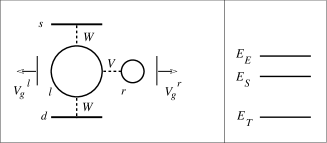
The capacitive energies in the left and right dots are different, $Q_{r}\gg Q_{l}$ so that the Coulomb blockade completely suppresses doubly occupied states in the right dot. The gate voltages $V_{g}^{l,r}$ are applied separately to the left and right dots. The new ingredient here is the introduction of a small ”trembling” (time dependent) component in the gate voltage of the right dot, so that

$$V_{g}^{r}=V_{g}^{r}(0)+v_{g}(t).$$

Let us first recall the spectrum of the TDQD in the absence of the time dependent component. The constant parts of the gate voltages are included in the energy levels of the double dot, $\epsilon_{l,r}=\varepsilon_{l,r}+V_{g}^{l,r}(0)$. These voltages are tuned in such a way that

$$\epsilon_{l}+\epsilon_{r}<2\epsilon_{l}+Q_{l}\ll 2\epsilon_{r}+Q_{r}.$$

Hereafter, the Fermi energy in the leads is chosen as the zero energy level. As excited states of the TDQD with two electrons in the right dot are excluded from the low-energy part of the spectrum, the low energy levels of the TDQD are KA01

$$E_{T}=\epsilon_{l}+\epsilon_{r}-M_{T},$$ (1)

$$E_{S}=\epsilon_{l}+\epsilon_{r}-2\beta V-M_{S},$$

$$E_{E}=2\epsilon_{l}+2\beta V+M_{E},$$

where $V$ is the potential which acts between the dots, see Fig.1. The notations $T,S,E$ respectively refer to triplet, singlet and exciton states of the TDQD. In the exciton state, the two electrons reside on the left dot. The above results are obtained in first order of the small parameter $\beta=V/(\varepsilon_{l}-\varepsilon_{r}+Q_{l})\ll 1$. Anticipating further analysis, we include in the low energy spectrum the level shifts $M_{\Lambda=T,S,E}$ which result from renormalization of the dot levels due to the tunnel contact with the leads (the so called ”Haldane renormalization” Hald , see below). It was shown in Ref. KA01, that $M_{T}>M_{S}$, so that the singlet and triplet levels may cross due to this renormalization. Such level crossing occurs provided the charge transfer exciton energy $E_{E}$ is not very high. Here we study just this regime, so that taking into account the above level renormalization, the ground state of the TDQD in a contact with the leads is a triplet state $E_{T}$ ( Fig. 1, right panel).

Having in mind the above energy level scheme (1) for the TDQD with constant gate voltages $V_{g}^{l,r}(0)$, we now consider the influence of the trembling potential $v_{g}(t)$ on the dot spectrum. As usual, one should discriminate between slow and fast components of a temporal perturbation and treat the former processes in an adiabatic approximation. In order to separate adiabatic and non-adiabatic parts of the trembling potential it is useful to introduce the spectral density $A(\Omega)$ of the trembling potential $v_{g}$:

$$v_{g}(t)=v_{g}\int d\Omega A(\Omega)e^{i\Omega t}.$$ (2)

In the present study we are mainly interested in the nearly adiabatic regime, where the spectral density is concentrated in the frequency interval $0<\Omega<\Omega_{a}$ with $\Omega_{a}\ll\Delta_{ST}=E_{S}-E_{T}$. In this case the contribution of the trembling potential may be treated by means of time-dependent scaling approach, while non-adiabatic corrections should be considered perturbatively.

The Hamiltonian describing the system schematically shown in Fig. 1 has the following form:

$$H=H_{band}+H_{dot}+H_{tun}.$$ (3)

Here the first term is the band Hamiltonian, which describes electrons in the leads [source ($s$) and drain ($d$), respectively],

$$H_{band}=\sum_{b=s,d}\varepsilon_{kb}c^{\dagger}_{kb\sigma}c_{kb\sigma}~{},$$ (4)

$k,\sigma$ are the wave vector and spin projection, respectively.

The tunneling Hamiltonian involves only electrons in the left dot.

$$H_{tun}=W\sum_{k\sigma}(c^{\dagger}_{k\sigma}d_{l\sigma}+H.c.),$$ (5)

where the operators $d_{l\sigma}$ correspond to electrons in the TDQD. In the tunneling part 5 we have already excluded one of the two channels from the tunneling Hamiltonian by introducing even and odd combinations of electron wave function in two leads. Then, only the even standing wave $c_{k\sigma}=\frac{1}{\sqrt{2}}(c_{ks\sigma}+c_{kd\sigma})$ enters $H_{tun}(0)$ (we consider a completely symmetric device with lead-dot tunneling constants $W_{s}=W_{d}=W$).

It is useful at this point to carry out some manipulations which will turn the discussion more transparent. In the first step, a canonical transformation is performed, BRUS ; GA ; KNG which eliminates the trembling potential from the diagonal part of the dot Hamiltonian

$$H_{dot}=H_{l0}+H_{lr0}+H_{r}~{},$$ (6)

with

$$H_{l0}=\varepsilon_{l}n_{l}+Q_{l}n_{l}^{2},$$

$$H_{lr0}=V\sum_{\sigma}(d_{l\sigma}^{\dagger}d_{r\sigma}+H.c.),$$

$$H_{r}=\varepsilon_{r}n_{r}+Q_{r}n^{2}_{r}+V_{g}(0)n_{r}+v_{g}(t)n_{r}=H_{r0}+H_{r}(t).$$

Here $n_{j}=d^{\dagger}_{j\sigma}d_{j\sigma}$ is the density operator for the electrons in the left $(j=l))$ and right ($j=r$) dot. The required transformation is,

$$\widetilde{H}=U_{1}HU_{1}^{-1}-i\hbar\frac{\partial U_{1}}{\partial t}U_{1}^{\dagger},$$ (7)

with $U_{1}\equiv\exp[-i\Phi_{1}(t)n_{r}]$ where the phase $\Phi_{1}(t)$ is given by

$$\Phi_{1}(t)=\frac{1}{\hbar}\int^{t}dt^{\prime}v_{g}(t^{\prime}).$$

This phase may be rewritten in terms of the spectral density introduced in Eq. 2:

$$\Phi_{1}(t)=\int d\Omega\Phi_{1}(\Omega)e^{i\Omega t}\equiv v_{g}\int d\Omega\frac{A(\Omega)}{(i\hbar\Omega)}e^{i\Omega t}.$$ (8)

Then, expanding the exponent in terms of the weak trembling potential, we come to the expression,

$$\tilde{H}_{dot} = H_{dot}^{(0)}+iV\Phi_{1}(t)\sum_{\sigma}(d^{\dagger}_{r\sigma}d_{l\sigma}-H.c.)$$ (9)

$$\equiv H_{dot}^{(0)}+H_{dot}(t)~{}.$$

In the next step, it proves to be more convenient to work in a representation $|\Lambda\rangle$, which diagonalizes the dot Hamiltonian, i.e. to rewrite it in terms of Hubbard operators $X^{\Lambda\Lambda^{\prime}}=|\Lambda\rangle\langle\Lambda^{\prime}|$. After the standard diagonalization procedure for the time independent part of the Hamiltonian we have KA01

$$H_{dot}^{(0)}=\sum_{\Lambda}E_{\Lambda}X^{\Lambda\Lambda},~{}~{}~{}~{}~{}~{}~{}~{}\Lambda=T\mu,S,E.$$ (10)

Recall again that $T,S,E$ stand for triplet, singlet and charge transfer exciton states of TDQD, respectively while $\mu=\pm 1,0$ are the spin projections of the triplet state. The diagonal Hubbard operators are constrained by the condition

$$\sum_{\Lambda}X^{\Lambda\Lambda}=1.$$ (11)

In terms of Hubbard operators the tunneling Hamiltonian (5) acquires the form

$$H_{tun}^{(0)}=W\sum_{\Lambda,\sigma\sigma^{\prime}}\left(c^{\dagger}_{k\sigma}X^{r_{\sigma^{\prime}}\Lambda}+H.c.\right).$$ (12)

Here the index $r_{\sigma^{\prime}}$ stands for the electron in the right well with spin projection $\sigma^{\prime}$, which remains in the TDQD, when the electron $l_{\sigma}$ escapes from the left well to the lead. As was mentioned above, the lead state $k\sigma$ means the even combination of lead electrons with the wave vector $k$. All tunneling transitions are described by the same constant $W$.

Writing $H_{dot}(t)$ from Eq. (9) in the form $H_{dot}(t)=iV\Phi_{1}(t){\cal S}_{lr}$ where

$${\cal S}_{lr}=\sum_{\sigma}(d^{\dagger}_{r\sigma}d_{l\sigma}-H.c.),$$

one finds

$${\cal S}_{lr}|S\rangle=\sqrt{2}|E\rangle,~{}~{}~{}{\cal S}_{lr}|E\rangle=-\sqrt{2}|S\rangle,~{}~{}~{}{\cal S}_{lr}|T\rangle=0.$$ (13)

It follows from these equations that

$${\cal S}_{lr}=\sqrt{2}(X^{ES}-X^{SE})\equiv iA\sqrt{2}.$$ (14)

The new scalar operator $A$ is one of the generators of the $SO(5)$ group, which characterizes the dynamical symmetry of a biased DQD (see Appendix A). Then, the commutation with the diagonal Hubbard operators yields

$$[{\cal S}_{lr},X^{SS}]=iA\sqrt{2},~{}~{}~{}[{\cal S}_{lr},X^{EE}]=-iA\sqrt{2}$$ (15)

(${\cal S}_{lr}$ is an anti-Hermitian operator). As a result, the GA transformation GA leads to

$$H_{dot}(t)=-\sqrt{2}V\Phi_{1}(t)A.$$ (16)

III Time-dependent poor man’s scaling

Next, the Haldane-Anderson scaling approach Hald should be applied to $H_{dot}+H_{band}+H_{tun}$ in order to rescale the energies in the TDQD. Here $H_{dot}$ (9) contains the time-dependent component. Unlike the static case considered in Ref. KA01, , we deal here with a TDQD whose Hamiltonian is non-diagonal in $\Lambda$, such that the off-diagonal elements are time-dependent. However, for the slow trembling potential with characteristic frequencies $\Omega_{a}\ll\Delta_{ES}=E_{E}-E_{S}$, one may treat this time-dependent term adiabatically at least in zero-order approximation. This means that before turning to the Haldane RG procedure, one has to get rid of the non-diagonal $SE$ mixing terms with the help of a second time-dependent canonical transformation. This transformation is given by the matrix $U_{2}=\exp\Theta$, which is found from the condition KNG

$$H_{dot}(t)+[\Theta,H_{dot}^{(0)}]=i\hbar\frac{\partial\Theta}{\partial t}.$$ (17)

Within the adiabatic approximation, one may carry out this diagonalization procedure at each moment $t$ neglecting any retardation and omitting the term in the r.h.s. of this equation. Then the matrix $\Theta$ is given by

$$\Theta=\frac{i\sqrt{2}V\Phi_{1}(t)}{\Delta_{ES}}(X^{ES}+X^{SE}).$$ (18)

At this stage, we apply the ”adiabatic” Haldane RG procedure, i.e. calculate the scaling trajectories of the energy states, which evolve with the reduction of the energy scale in the metallic reservoir from the initial value $D_{0}$ to the actual value $D$. Since the transformations (7) and (17) do not involve the triplet state, the scaling trajectory $E_{T}$ as a function of scaling variable $\xi=\ln(D_{0}/D)$ is the same as in our previous calculations. KA01 As a result, the triplet state includes only the time-independent Haldane shift, whereas the two singlet states acquire time dependence,

$$E_{T} \to E_{T}-M_{T}(\xi),$$ (19)

$$E_{S}(t) \to E_{S}-M_{S}(\xi)-C_{S}\Phi_{1}^{2}(t),$$

$$E_{E}(t) \to E_{E}+M_{E}(\xi)+C_{S}\Phi_{1}^{2}(t).$$

Here $C_{S}={2V^{2}}/\Delta_{ES}$ is an additional time-dependent adiabatic part within the Haldane renormalization scheme. Thus, the term $H_{dot}^{(0)}$ in the dot Hamiltonian (9) is given by Eq. (10) and

$$H_{dot}(t)=C_{S}\Phi_{1}^{2}(t)(X^{EE}-X^{SS}).$$ (20)

There is no correction to the matrix $\Theta$ from the time derivative in the r.h.s. of Eq. (17) at least up to first order in the adiabatic parameter $\kappa_{1}=v_{g}(t)/\Delta_{ES}$. Besides, due to the same transformation $U_{2}$, the components of the tunnel Hamiltonian containing operators $X^{E\lambda}$ and $X^{S\lambda}$ become time dependent as well,

$$H_{tun}=H_{tun}^{(0)}+H_{tun}(t).$$ (21)

The ”trembling tunneling” contribution in these terms has the form

$$H_{tun}(t)=-i\sqrt{2}\frac{VW\Phi_{1}(t)}{\Delta_{ES}}\sum_{k\sigma}(X^{Sr_{\bar{\sigma}}}+X^{Er_{\bar{\sigma}}})c_{k\sigma}-H.c.$$ (22)

Thus, the trembling gate voltage generates time-dependent tunneling through the singlet states, but the operator form of $H_{tun}$ is conserved.

We see that the trembling potential involves a contribution of the excited singlet in the tunneling Hamiltonian, and the latter introduces fluctuations in tunneling through the ground state singlet. The spin $S=1$ states are not involved in these trembling processes. However, eventually we expect that the triplet is subject to dephasing via the operators ${\bf P}$ and ${\bf M}$ (see equation LABEL:SW2 below) due to dynamical $SO(5)$ symmetry of the TDQD (see Appendix A). One should remember that the state $|E\rangle$ enters the manifold of eigenstates of the isolated TDQD (10). In the static case this high energy charge excitation is admixed with the low-lying singlet spin state $|S\rangle$. This admixture changes the lead-dot tunneling rate and can lead to the inequality $M_{T}>M_{S}$ mentioned earlier. We consider the situation well beyond the S/T crossover so that the positive singlet-triplet energy gap satisfies the inequality $\Delta_{ST}=E_{S}-E_{T}\gg\Omega_{a}$. The adiabatic Haldane procedure (19) results in a time-dependent S/T energy gap

$$\Delta_{ST}(t)=E_{S}-E_{T}-\delta(t),$$

$$\delta(t)=C_{S}\Phi_{1}^{2}(t).$$ (23)

The adiabatic contribution of a charge transfer exciton $(E)$ to the effective indirect exchange (cotunneling) Hamiltonian may be taken into account by means of a time dependent Schrieffer-Wolff transformation, which includes $H_{tun}(t)$ (22). This transformation is described in Ref. KNG, for the dot occupied by a single electron with $S=1/2$. In our case the exchange Hamiltonian is affected by the trembling perturbation in spite of the fact that the localized spin ${\bf S}=1$ is not directly affected by the time dependent potential. However, charge fluctuations induced by time dependent tunneling (22) perturb the $S$- and $E$-states, which are connected with the spin by the kinematics of vector and scalar operators of the dynamical symmetry group $SO(5)$. All these corrections can be incorporated in the Schrieffer-Wolff (SW) Hamiltonian $H_{SW}$ for the dot obeying the SO(5) symmetry. The time-independent part of the SW Hamiltonian takes the form KKA

$$H_{SW}^{(0)} = H_{dot}^{(0)}+H_{cotun}^{(0)},$$ (24)

$$H_{dot}^{(0)} = \frac{1}{2}\left(E_{T}{\bf S}^{2}+E_{S}{\bf P}^{2}+E_{E}{\bf M}^{2}\right)+Q({\hat{N}}-2)^{2},$$

$$H_{cotun}^{(0)} = J^{T}_{0}{\bf S}\cdot{\bf s}+J^{ST}_{0}{\bf P}\cdot{\bf s}+J^{ET}_{0}{\bf M}\cdot{\bf s}.$$

Here the terms describing the irrelevant potential scattering are omitted (see, however, the discussion of fluctuation corrections in Section IV).

The Hamiltonian (24) is expressed in terms of SO(5) group generators presented in Appendix A. Here $\hat{N}$ is the operator of particle occupation number, and the last term in (24) describes the constraint $N=2$ imposed by the Coulomb blockade $Q$ on the charge sector of the Hilbert space. As we mentioned already, the operator ${\bf S}$ is not affected by the time-dependent canonical transformations. However, the operators ${\bf P}$ and ${\bf M}$ will be involved in the time-dependent processes.

We generalize the adiabatic SW transformation derived in Ref. KNG, by introducing the matrix $U_{3}=\exp i\Upsilon$ with $\Upsilon$ defined as

$$\Upsilon(t)=\sum_{k\sigma}\left[\upsilon_{k}^{S}(t)X^{Sr_{\bar{\sigma}}}c_{k\sigma}+\upsilon_{k}^{E}(t)X^{Er_{\bar{\sigma}}}c_{k\sigma}-H.c.\right].$$ (25)

The coefficients $\upsilon_{k}^{\Lambda}$ are chosen to eliminate the time dependent terms (22) in the effective Hamiltonian

$$H_{SW}=\exp(-i\Upsilon)[H_{dot}+H_{band}+H_{tun}]\exp i\Upsilon,$$ (26)

where the first and third terms in the Hamiltonian depend on time. To fulfil this request, the transformation matrix should satisfy the equation

$$H_{tun}+[\Upsilon,(H_{dot}+H_{band})]=i\hbar\frac{\partial\Upsilon}{\partial t}$$ (27)

(cf. Eq. 17). Repeating the procedure used in the calculation of the matrix $U_{2}$ and including the first order corrections in the adiabaticity parameters $\kappa_{2}^{S}(t)=v_{g}(t)/\epsilon_{l}$ and $\kappa_{2}^{E}(t)=v_{g}(t)/(2\epsilon_{l}-\epsilon_{r})$ from the time derivative on the r.h.s. of Eq. (27), one finds the following expression for $\Upsilon(t)$

$$\Upsilon(t)=\Upsilon_{T}+\Upsilon_{S}(t)+\Upsilon_{E}(t),$$ (28)

$$\Upsilon_{T}=\frac{W}{\epsilon_{l}-M_{T}}\sum_{k\sigma\sigma^{\prime}}\sum_{\nu=0,1,\bar{1}}\left(X^{\nu,r\sigma^{\prime}}c_{k\sigma}-H.c.\right),$$

$$\Upsilon_{S}(t)=\frac{W-w_{2}^{S}(t)}{\epsilon_{l}-M_{S}(t)}\sum_{k\sigma}(X^{S,r_{\bar{\sigma}}}c_{k\sigma}-H.c.),$$

$$\Upsilon_{E}(t)=\frac{W-w_{2}^{E}(t)}{2\epsilon_{l}-\epsilon_{r}+M_{E}(t)}\sum_{k\sigma}(X^{E,r_{\bar{\sigma}}}c_{k\sigma}-H.c.).$$

The time-dependent quantities in $\Upsilon_{S}$ and $\Upsilon_{E}$ are

$$M_{S}(t)=M_{S}-C_{S}\Phi_{1}^{2}(t),\;\;\;M_{E}(t)=M_{E}+C_{S}\Phi_{1}^{2}(t)$$

$$w_{2}^{S}(t)=\frac{VW\sqrt{2}\Phi_{2}^{S}(t)}{\Delta_{ES}},\;\;\;w_{2}^{E}(t)=\frac{VW\sqrt{2}\Phi_{2}^{E}(t)}{\Delta_{ES}},$$

with $\Phi_{2}^{S}(t)=\Phi_{1}(t)-\alpha_{2}^{S}(t)$ and $\Phi_{2}^{E}(t)=\Phi_{1}(t)-\alpha_{2}^{E}(t)$.

This procedure results in the appearance of a time-dependent component in $H_{cotun}$, which modifies the coupling constants $J^{ST}$ and$J^{ET}$ in the Hamiltonian (24). As a result, we get the following effective exchange Hamiltonian which induces the decoherence and dephasing effects in the Kondo tunneling through TDQD:

$$H_{cotun} = J^{TT}_{0}{\bf S}\cdot{\bf s}+J^{ST}(t){\bf P}\cdot{\bf s}+J^{ET}(t){\bf M}\cdot{\bf s}.$$

Here

$$J^{ST}(t)=\frac{W-w_{2}^{S}(t)}{\epsilon_{l}-M_{S}(t)}\cdot\frac{W(1-V/\Delta_{ES})\sqrt{2}\Phi_{1}(t)}{\Delta_{ES}},$$ (30)

$$J^{ET}(t)=\frac{W-w_{2}^{E}(t)}{2\epsilon_{r}-\epsilon_{l}+M_{E}(t)}\cdot\frac{W(1-V/\Delta_{ES})\sqrt{2}\Phi_{1}(t)}{\Delta_{ES}},$$ (31)

and the time-dependent parts of the coupling constant $J^{ST}$ and $J^{ET}$ may be obtained by expansion of its general form in the adiabatic parameters $\kappa_{1},\kappa_{2}^{S},\kappa_{2}^{E}$.

The first manifestation of this time dependence, which can be seen already within an adiabatic approximation is the uncertainty in the definition of the Kondo temperature. To describe this effect, we refer to the poor man’s scaling equations for the Kondo effect in DQD for time-independent Hamiltonian (24) derived previously. KA01 In the adiabatic regime, these equations retain their form, but the coupling constants depend on time $t$ as a parameter. In particular in the limit when the exciton state $|E\rangle$ is quenched, the system of scaling equations has the form

$$dj_{1}/d\xi=-j_{1}^{2}-[j_{2}(t)]^{2};~{}~{}~{}dj_{2}/d\xi=-2j_{1}j_{2}(t).$$ (32)

Here $j_{1}=\rho_{0}J^{TT},~{}j_{2}=\rho_{0}J^{ST},~{}j_{3}=\rho_{0}J^{ET}$, $\rho_{0}$ is the density of states at the Fermi level.

As is already established in the theory of Kondo-effect at a singlet-triplet (S/T) crossing,KA01 ; GT01 ; Pust1 ; Eto in the limit $\Delta_{ST}\gg T_{K}$ the solution of these equations may be expressed in terms of $T_{K0}=D_{0}\exp[-1/(j_{1}+j_{2})]$:

$$\frac{T_{K}}{T_{K0}}=\left[\frac{T_{K0}}{\Delta_{ST}(t)}\right]^{\zeta},$$ (33)

where $\zeta\lesssim 1$ is a constant. The relative amplitude $\delta T_{K}$ of adiabatic variations of the ”time-dependent Kondo temperature” KNG may be estimated from this equation:

$$\delta T_{K}\approx\left[\frac{T_{K0}}{\Delta_{ST}(0)}\right]^{1+\zeta}2C_{S}\Phi_{1}^{2}$$ (34)

($\Phi_{1}^{2}$ is the mean square value of the trembling parameter). In this asymptotic region, the time-dependent corrections are insignificant. In accordance with the above mentioned theory of an S/T transition for a time-independent gate voltage,KA01 ; GT01 ; Pust1 ; Eto the Kondo temperature increases with decreasing $\Delta_{ST}$ and reaches its maximum $T_{K}=T_{K0}$ at a crossing point $\Delta_{ST}=0$. One may expect that the role of non-adiabatic corrections increases with decreasing $\Delta_{ST}$. As a result, the scaling behavior should be seriously violated when approaching the crossing point, and the deviations from the prescriptions of an adiabatic theory in the dependence $T_{K}(\Delta_{ST})$ should grow accordingly.

IV Fluctuation corrections to RG equations

In this section we go beyond the adiabatic approximation and take into account decoherence and dephasing corrections to the Kondo tunneling. Unlike the mechanisms described in Ref. KNG, , where the time-dependent spin-flip processes were the source of dephasing, we appeal here to gauge fluctuations, which arise because two singlet states $|S\rangle$ and $|E\rangle$ are involved in the formation of a Kondo resonance in a triplet ground state $|T\rangle$ in the process of time-dependent cotunneling.

The first source of non-adiabatic corrections is associated with the fluctuations of the energy gap $\Delta_{ST}$ (23), which may be converted into gauge fluctuations of a Casimir operator (68). Using an obvious chain of subsets,

$$U(1)\subset SU(2)\subset SO(4)\subset SO(5),$$

we conclude that the trembling potential affects the least continuous subgroup of $SO(5)$.

To perform this conversion we turn to the fermionic representation of the generators of the $SO(5)$ group (see Appendix A). We now work in the subspace of low-energy states $|T\rangle,|S\rangle$, which are described by the dynamical symmetry group $SO(4)$. Then the non-adiabatic fluctuations of the energy gap $\Delta_{ES}$ may be described as fluctuations of the ”reduced” Casimir operator ${\bf S}^{2}+{\bf P}^{2}$, which, in turn is rewritten as a local constraint (71) where the last term is eliminated. We introduce the ”fluctuating constraint” in $H_{dot}$ by means of a time-dependent Lagrange factor $\mu$:

$$H_{dot}^{\prime}=H_{dot}(0)-\mu(t)(\hat{R}-1)$$ (35)

with

$$\hat{R}=f^{\dagger}_{s}f_{s}+\sum_{\nu=1,0,\bar{1}}f^{\dagger}_{\nu}f_{\nu}~{}.$$

Thus, the fluctuating constraint takes into account time-dependent admixture of the $E$-state to the $S$-state. Although the exciton $E$ is excluded from the effective spin space, its effects are present through a ”randomization” of the constraint. The fluctuating time-dependent Lagrange factor can be eliminated from the $SO(4)$ fermionic Green’s functions by means of the global $U(1)$ gauge transformation performed in all sectors of the $f$-representation

$$f_{\lambda}\to f_{\lambda}e^{i\phi(t)}.$$ (36)

Minimizing the free fermion part of the Lagrangian, one has $\hbar\dot{\phi}(t)=\mu(t)$ (here $\lambda=\bar{1},0,1,s$).

On the other hand, the constraint fluctuations in terms of time-dependent Lagrange factors can be reformulated as a propagation of fermions along the time axis in the presence of a time-dependent external scalar potential. The solution of this problem results in the appearance of an imaginary part in the zero frequency spin fermion propagators, ${\rm Im}\Sigma_{f}(0)=\gamma$ (see below). Eventually, the existence of this damping prevents the formation of a coherent Kondo tunneling regime through DQD at zero temperature, so the effects connected with this type of gauge fluctuations can be qualified as decoherence.

Another source of non-adiabatic gauge fluctuations comes from the time-dependent poor man’s scaling solution. The co-tunneling Hamiltonian (31) contains the time-dependent corrections to ${\bf P\cdot s}$ and ${\bf M\cdot s}$. In this case (unlike the first mechanism), the source of gauge fluctuations is due to non-diagonal operators P, M, so that the time-dependent coupling constants are parametrized as $j_{2}(t)=j_{2}e^{i\theta_{ST}(t)}$ and $j_{3}(t)=j_{3}e^{i\theta_{ET}(t)}$.

The phases in $j^{\Lambda\Lambda^{\prime}}$ can be eliminated by the local $U(1)$ gauge transformation

$$f_{\lambda}\to f_{\lambda}e^{i\vartheta_{\lambda}(t)}$$ (37)

performed in the $S$-, $T$- and $E$-sectors of the fermionic representation of the $SO(5)$ group. The local gauge phases may be represented as

$$\theta_{ST}(t)=\vartheta_{T}(t)-\vartheta_{S}(t),\;\;\theta_{ET}(t)=\vartheta_{T}(t)-\vartheta_{E}(t)$$ (38)

so that the phases $\vartheta_{\lambda}(t)$ have different time derivatives. Therefore, the effects related to this type of gauge fluctuations are, in fact, dephasing effects stemming out of weakly non-adiabatic $TS$ and $TE$ transitions.

Now we turn to the calculation of gauge fluctuation corrections in the self energies and vertices entering the Kondo tunneling diagrams. To calculate the damping of retarded spin-fermion propagators in the triplet sector of phase space

$$G_{T\mu}(t-t^{\prime})=\langle f_{\mu}(t)f^{\dagger}_{\mu}(t^{\prime})\rangle_{R}=-i\langle[f_{\mu}(t)f^{\dagger}_{\mu}(t^{\prime})]_{+}\rangle$$ (39)

we apply perturbation theory for time-dependent external potentials to the last term in the Hamiltonian (35). In the corresponding diagrammatic technique the times $t$ are marked by crosses and the correlation functions connecting the fluctuations related to the instants $t,t^{\prime}$ are denoted by wavy lines. Then the first order diagram for the self energy of $G_{T\mu}(t-t^{\prime})$ is given by the diagram Fig. 2 (the spin-fermion propagator is represented by the full line). We consider the simplest case of white-noise correlations $\hbar^{2}\langle\dot{\phi}_{1}(t)\dot{\phi}_{1}(t^{\prime})\rangle=r_{0}\delta(t-t^{\prime}).$

Figure 2: Self energy correction due to gauge fluctuations in spin-fermion propagator.

The corresponding contribution to the self energy is a purely imaginary damping

$$\gamma_{1}=\hbar/2\tau_{d}\sim C_{S}^{2}r_{0}.$$ (40)

This first order approximation is valid as long as the damping is weak in comparison with the Kondo temperature, $\hbar/\tau_{d}\ll T_{K}$. If these two quantities are comparable then the whole sequence of ”rainbow” diagrams should be inserted in the spin-fermion self energy. This means that instead of the white noise we get a more realistic description of trembling, which takes the retardation effects (non-gaussian corrections) into account. This specification is not too essential for our purposes. More important is the low-energy cutoff $\sim\hbar/\tau_{d}$ in the RG procedure, which prevents crossover to the strong-coupling limit of the Kondo tunneling due to incoherent phase fluctuations.

Our next goal is to find non-adiabatic corrections for exchange vertices, which contribute to the dephasing mechanism mentioned above (see Eq. 38). Dephasing means that the gauge transformation (37) eliminates the phase $\theta_{ST}$ within the accuracy of phase fluctuations, i.e. the local gauge phases have the form

$$\theta_{ST}(t)=\vartheta_{T}(t)-\vartheta_{S}(t)+\varphi_{s}(t),$$

$$\theta_{ET}(t)=\vartheta_{T}(t)-\vartheta_{E}(t)+\varphi_{e}(t).$$ (41)

Then, expanding the exponents in the non-adiabatic vertex corrections $J^{ST}\left[e^{i\varphi_{s}(t)}-1\right]$ and $J^{ET}\left[e^{i\varphi_{e}(t)}-1\right]$, we obtain the fluctuating part of the Hamiltonian (LABEL:SW2) in a form

$$\delta H_{cotun}=i\left[J^{ST}\varphi_{s}(t){\bf P}\cdot{\bf s}+J^{ET}\varphi_{e}(t){\bf M}\cdot{\bf s}\right].$$ (42)

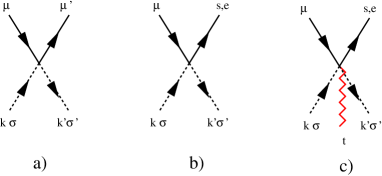
Adiabatic vertices (24) and non-adiabatic corrections (42) may be presented in a graphical form (Fig. 3). The bare interactions are shown in Figs. 3(a,b) by means of four-tail vertices where the operators ${\bf S}$, ${\bf P}$ and ${\bf M}$ are expressed via fermion operators in accordance with Eqs. (A). Here solid lines stand for spin fermions and dashed lines represent conduction electrons.

The time-dependent vertices (42) are shown in Fig. 3c, where the broken line stands for the fluctuation field $D(t)=\langle\varphi(t)\varphi(0)\rangle_{R}$.

Figure 3: (a) Adiabatic exchange vertices for triplet channel $T$; ( b) Similar diagrams for $ST$ and $ET$ channels; (c) non-adiabatic corrections to two latter vertices.

If the fluctuating trembling signal is characterized by retardation,

$$D(t)=-i\alpha^{2}e^{-\zeta|t|}$$ (43)

then the Fourier transform of this correlation function is

$$D(\omega)=\frac{2i\alpha^{2}\zeta}{\omega^{2}+\zeta^{2}}.$$ (44)

Other elements entering the vertices are $G_{T\nu}(t-t^{\prime})$ defined in Eq. (39), a similar propagator for spinless fermions representing the singlet state

$$G_{S}(t-t^{\prime})=\langle f_{s}(t)f^{\dagger}_{s}(t^{\prime})\rangle_{R}.$$ (45)

and conduction electron propagators

$$g_{k\sigma}(t-t^{\prime})=\langle c_{k\sigma}(t)c^{\dagger}_{k\sigma}(t^{\prime})\rangle_{R}.$$ (46)

The Fourier transforms of the Green functions (39), (45) and (46) are

$$G_{T\mu}(\omega) = (\omega+i\eta)^{-1},~{}~{}G_{S}(\omega)=(\omega-\Delta_{TS}+i\eta)^{-1},$$ (47)

$$g_{k\sigma}(\omega)=(\omega-\varepsilon_{k\sigma}+i\eta)^{-1}.$$

(here $\eta\to+0$).

The first fluctuation correction to adiabatic vertices Fig. 4a is displayed in Fig. 4b.

Figure 4: First leading parquet diagram (a) and first non-adiabatic correction to it (b). The pseudofermion, electron and fluctuation propagators are represented by solid, dotted and broken lines, respectively. The absence of direction in electron propagator lines assumes that both directions (clockwise and anti-clockwise) are possible.

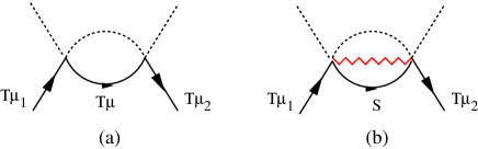
Although the contribution of the diagram in Fig. 4b is parametrically small compared with that of Fig. 4a due to a small factor $(\alpha j_{0}^{ST})^{2}\ll 1$, this diagram represents a building block for construction of non-adiabatic corrections for vertices and self-energy parts. These corrections affect both adiabatic vertices (see Appendix B) and the self energy $\Sigma_{T}(\omega)$ of the spin-fermion propagator $G_{T\mu}$ (Fig. 5). The latter diagram may be obtained from the vertex (Fig.4b) by gluing two free electron lines in the electron propagator. Besides, the diagram (Fig. 5) is connected with first non-parquet TT vertex by a Ward identity (see Appendix B). We will use this identity below, when calculating the spin relaxation corrections.

Figure 5: First non-adiabatic correction to propagator $G_{T\mu}$.

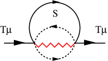
The imaginary part of the self-energy Fig. 5 is given by the following expression

$$\frac{\hbar}{\tau_{T}(\omega)}={\rm Im}\Sigma_{T}(\omega)=(\alpha j_{2})^{2}\times$$ (48)

$$\int\int d\varepsilon_{1}d\varepsilon_{2}{\rm Im}K_{\sigma_{l}\sigma_{2}}^{(R)}(\varepsilon_{1}-\varepsilon_{2}){\rm Im}D(\omega-\varepsilon_{1}){\rm Im}G_{S}^{(R)}(\varepsilon_{2})$$

$$\left(\tanh\frac{\varepsilon_{2}}{2T}+\coth\frac{\varepsilon_{1}-\varepsilon_{2}}{2T}\right)\left(\tanh\frac{\varepsilon_{1}}{2T}+\coth\frac{\omega-\varepsilon_{1}}{2T}\right).$$

We assume that the decrement $\gamma$ in the propagator $D(t)$ (43) is small in comparison with the energies $\Delta_{ST}$ and $\Delta_{ET}$ since we remain in the weakly non-adiabatic regime. Here $K^{R}(\omega)$ is the Fourier transform of the spin susceptibility of the electron gas in the leads

$$K^{R}(t-t^{\prime})=\sum_{k_{1}k_{2}k_{3}k_{4}}\langle c^{\dagger}_{k_{1}\sigma_{1}}(t)c_{k_{2}\sigma_{2}}(t)c^{\dagger}_{k_{3}\sigma_{2}}(t^{\prime})c_{k_{4}\sigma_{1}}(t^{\prime})\rangle_{R}$$

which may be expressed via convolution of two electron propagators,

$$K^{R}(t-t^{\prime})=\sum_{kq}g_{k\sigma_{1}}(t-t^{\prime})g_{k+q,\sigma_{2}}(t^{\prime}-t).$$

The actual frequency interval is very narrow in comparison with the electron Fermi energy, $\omega\ll\varepsilon_{F}$). At low frequencies the Fourier transform of the electron-hole polarization loop $K^{R}(\omega)$ behaves as

$${\rm Im}\;K^{R}(\omega)\sim\rho_{0}\frac{\omega}{\varepsilon_{F}}~{}.$$

Using this relation, one may estimate the dephasing rate:

$$\gamma_{2}=\frac{\hbar}{2\tau_{T}(\omega\to 0)}\sim\left({\alpha j_{2}}\right)^{2}\left\{\begin{array}[]{ll}\displaystyle\Delta_{ST}e^{-\Delta_{ST}/T},~{}~{}T<\Delta_{ST}\\ \\ \displaystyle\frac{T^{2}}{\Delta_{ST}},~{}~{}\Delta_{ST}<T<\Delta_{ET}\end{array}\right.$$ (51)

We see that this contribution to the dephasing effect is frozen out at low temperatures because the singlet states responsible for dephasing is depopulated at $T\ll\Delta_{TS}$.

Now the self-energy corrections to the spin-fermion propagator $G_{T\mu}$ represented by the diagrams Fig. 2 and Fig. 5 may be used in the scaling equations (32). As a result of fluctuation corrections, $G_{T\mu}$ acquires the form

$$G_{T\mu}(\omega)=(\omega+i\gamma)^{-1},$$ (52)

where $\gamma=\gamma_{1}$ at $T\to 0$ and $\gamma=\gamma_{2}$ at $T\to\Delta_{ST}$. These propagators should be inserted in the diagrams arising in the poor man’s scaling procedure anders (the first of these diagrams is shown in Fig. 4). Then we immediately conclude that this imaginary part transforms into the infrared cutoff of Kondo singularity. This means that there is no significant effect of fluctuations on Kondo tunneling at high $T\sim\Delta_{ST}$ provided $\gamma_{2}\ll T_{K}$, where $\gamma_{2}\sim T^{2}/\Delta_{ST}$. However both dephasing and decoherence prevent the achievement of the unitarity limit at $T\to 0$.

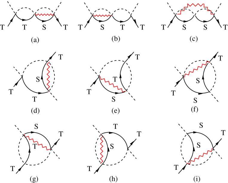
Our last task is to clarify the contribution of vertex corrections presented in Figs. 4b, 6 and 7 to the scaling equations (32). It is clear that the real parts of these corrections only slightly renormalize the coupling parameters $j_{1,2}$ and do not influence the scaling trajectories. As to the imaginary part $\Gamma^{{}^{\prime\prime}}_{TT}$, it determines the longitudinal $1/T_{1}$ and transverse $1/T_{2}$ relaxation rates by means of the correlation function,

$$\chi_{t}(\omega)=\langle{\bf S},{\bf S}\rangle_{R}$$ (53)

which can be interpreted as line-shape. While all diagrams Fig.6 a-i contribute both to $1/T_{1}$ and $1/T_{2}$ relaxation rates, the diagram Fig.7.a corresponds only to scattering processes without spin flip, resulting in slightly different temperature behavior of longitudinal and transverse relaxation rates. We note, however, that the difference between $1/T_{1}$ and $1/T_{2}$ appears only beyond the leading logarithmic approximation.

The imaginary part $\Gamma^{{}^{\prime\prime}}_{ST}$ is associated with spin relaxation processes determined by the specific kind of dynamical spin susceptibility

$$\chi_{st}(\omega)=\langle{\bf P},{\bf P}\rangle_{R}~{}~{},$$ (54)

which describes the response of a magnetic system with $SO(n)$ symmetry not to external magnetic field but to the perturbations intermixing triplet and singlet components of the spin manifold [including gauge fluctuations (41)]. This correlator, given by the irreducible S/T loop (see Fig.7.b-d) leads to the appearance of a new $1/T_{3}$ relaxation rate associated with the inverse time of transitions between the singlet and the 3-fold degenerate triplet state.

The diagrams (a,b,d,e,g,h) presented in the first two columns of Fig. 6 are in fact taken into account in the RG equations together with the diagram (Fig. 4b). Each of the three diagrams (c,f,g) in the last column of Fig. 6 contains two singlet propagators $G_{S}(\epsilon)$, so one should consider them together with the non-parquet diagram (Fig. 7a). This vertex correction to $J_{0}^{TT}$ together with non-logarithmic corrections (Fig. 7b-d) due to fluctuation induced $(T\to S\to T...)$ transitions accompany the adiabatic $TT$- and $ST$-exchanges and introduce the longitudinal and transversal spin relaxation times in the RG procedure (cf. Refs. KNG, ; Paas, ).

The fluctuation induced vertex correction (Fig. 7a) may be estimated with the help of the Ward identity for $G_{S}(\omega\to 0)$ written in the form

$$\left.\frac{\partial\Sigma_{TT}}{\partial\Delta_{TS}}\right|_{\omega\to 0}=\Gamma_{TT}(0),$$ (55)

where $\Sigma_{TT}$ is the self energy shown in Fig. 5 and $\Gamma_{TT}$ is the triplet vertex (Fig. 7.(a)). The Ward identity in this context corresponds to spin conservation in the process of quasi-elastic scattering. We conclude from these estimates that the non-adiabatic corrections $\hbar/(2\tau_{TT})=Im\Gamma_{TT}$ presented by the diagram Fig. 7.(a) are exponentially weak at low $T\ll\Delta_{ST}$ similarly to the dephasing rate $\gamma_{2}$.

Let us now consider the fluctuation corrections to the vertex $J^{ST}$ represented in Fig. 7.b-d. There is no Ward identity for this inelastic process, which does not conserve spin projection, so we calculate the vertex $\Gamma_{ST}$ straightforwardly with the help of Eq.(C). The imaginary part of the diagram Fig. 7b gives the following correction to $\Gamma_{ST}(\omega,0)$ at $\omega\approx\Delta_{ST}$ (see Appendix B):

$${\rm Im}[\rho_{0}\Gamma_{ST}^{(b)}]=\left(\alpha^{2}j_{2}^{3}\right)\left\{\begin{array}[]{ll}\displaystyle T/\Delta_{ST},~{}~{}\Delta_{ST}<T<\Delta_{ET}\\ \\ \displaystyle\omega/\Delta_{ST},~{}~{}T<\Delta_{ST}\end{array}\right.$$ (59)

The estimates of the next diagrams Fig. 7c,d give a similar result. Such behavior of non-diagonal vertex corrections is predetermined by the threshold character of T/S excitations at finite frequency. kis03

These vertex corrections should be inserted in the scaling equations (32). The imaginary part of the exchange vertex introduces an additional cutoff in the scaling procedure. Paas Taking into account the fact that the contribution of the singlet state to the flow equations controlled by the vertex $j_{2}$ is frozen for $D<\Delta_{ST}$, one immediately finds that the relaxation processes practically do not influence the cutoff of $j_{2}$ because

$$\hbar/(2\tau_{ST})={\rm}{\rm Im}\Gamma_{ST}(\omega=\Delta_{ST})\ll\Delta_{ST}.$$ (60)

The real part

$${\rm Re}[\rho_{0}\Gamma_{ST}]\sim\left(\alpha^{2}j_{2}^{3}\right)(T/\Delta_{ST})\ln(D/T),$$ (61)

just slightly disturbs the flow trajectories. Hence, it may also be neglected in perturbative estimates.

As in the case of non-equilibrium Kondo effectPaas , the spin-relaxation processes are controlled by the imaginary part of the susceptibility $K^{R}(\omega)$ of the electron liquid in the leads. However, in our case the susceptibility is moderated by the gauge fluctuations (broken line insertions in the electron-hole or singlet-triplet loops in Fig. 7(a-d)). As a result, the relaxation corrections do not affect Kondo tunneling at least in the weakly non-adiabatic regime.

V Conclusion

A double quantum dot with a weak trembling potential applied to the right dot (Fig. 1a) turned out to be an excellent model system in which all facets of decoherence phenomenon are exposed as observable effects. From a theoretical point of view, this system is especially attractive because decoherence, dephasing and relaxation are induced by the same gauge fluctuations, which develop in the constrained Hilbert space of the spin manifold $\{T,S,E\}$ (Fig. 1b) coupled to a Fermi bath of conduction electrons. All these processes may be discussed in a general context of the theory of decoherence in quantum systems in contact with a thermal bath.

The decoherence effect characterized by the time $\tau_{d}$ (40) is related to the structure of the ground state of TDQD in contact with the Fermi bath. It may be interpreted in terms of the Superselection Rule introduced by Wick, Wightman and Wigner for the description of baryonic charge (see Ref. Wight, for a recent review). Indeed, there is no symmetry ban for superposition of two singlet states $|S\rangle$ and $|E\rangle$, but this superposition arises only as a result of the coupling of the TDQD with the Fermi bath. The covering group, which describes the symmetry of the manifold $\{T,S,E\}$ is $SO(5)$, and the dynamical superposition is controlled by $U(1)$ gauge fluctuations (36) under the Casimir constraint (71). Due to these fluctuations, the coherent Kondo-type ground state of the system ’TDQD + Fermi bath’ cannot be reached.

The dephasing effect characterized by the time $\tau_{T}$ stems from the phase averaging in thermodynamical ensemble at finite temperature. Dephasing $\theta_{ST},\theta_{ET}$ (38) emerge in a process of exchange scattering induced by the random trembling potential. The scattering probabilities are added incoherently, so that the spin-fermion self energy acquires an imaginary part (Fig. 5). Such processes are generally classified as decoherence induced by dressing of bare states.Zeh

The relaxation effects characterized by the times $\tau_{TT}$ and $\tau_{ST}$ remind those known in the conventional theory of spin relaxation. Although we describe them in terms of triplet-triplet and triplet-singlet transitions, one may reinterpret the same processes in terms of longitudinal, transversal and S/T relaxation rates $1/T_{1}$, $1/T_{2}$ and $1/T_{3}$ because both $TT$ and $TS$ processes contain spin conserving and spin reversal components [see Eqs. (A)]. However, since all these processes are controlled by the small coupling constant $\left({\alpha j_{2}}\right)^{2}$ induced by the trembling potential, the relaxation contribution to dephasing processes is ineffective.

To conclude, we have shown in this paper that charge fluctuations can be transformed into spin fluctuations, which result in decoherence and dephasing of the Kondo effect in the double quantum dot system. All these phenomena arise due to intrinsic dynamical $SO(5)$ symmetry of the spin multiplet. Although we considered only a weakly non-adiabatic regime where decoherence effects are small by definition, the results are instructive, because one may strictly discriminate between pure decoherence of the ground state and the finite temperature dephasing and relaxation effects in a situation, where all these effects are due to gauge fluctuations within a spin multiplet. Strongly non-adiabatic response to trembling gate potential demands special consideration.

Appendix A Lie algebra for asymmetric DQD

If the excitonic state is included in the set of the energy levels, then the transitions between different states are described by the $o_{5}$ algebra. In addition to standard $S=1$ operators

$$S^{+} = \sqrt{2}\left(X^{10}+X^{0,-1}\right),~{}S^{-}=\sqrt{2}\left(X^{01}+X^{-1,0}\right),$$

$$S_{z} = X^{11}-X^{-1,-1},$$ (62)

one should introduce two more vectors. The vector ${\bf P}$ with the spherical components

$$P^{+} = \sqrt{2}\left(X^{1S}-X^{S,-1}\right),\;P^{-}=\sqrt{2}\left(X^{S1}-X^{-1,S}\right),$$

$$P_{z} = -\left(X^{0S}+X^{S0}\right).$$ (63)

defines transitions between the singlet $|S\rangle$ and the components $|T\mu\rangle$ of spin triplet. Similarly, the vector ${\bf M}$ with components

$$M^{+} = \sqrt{2}\left(X^{1E}-X^{E,-1}\right),\;M^{-}=\sqrt{2}\left(X^{E1}-X^{-1,E}\right),$$

$$M_{z} = -\left(X^{0E}+X^{E0}\right).$$ (64)

determines transitions between the left exciton and the triplet. The $o_{5}$ algebra is completed by the operator $A$

$$A=-i(X^{ES}-X^{SE}).$$ (65)

The Lie algebra is defined by the following commutation relations

$$[S_{j},S_{k}]=ie_{jkl}S_{l},\;\;[P_{j},P_{k}]=ie_{jkl}S_{l},\;\;[P_{j},S_{k}]=ie_{jkl}P_{l},$$

$$[M_{j},M_{k}]=ie_{jkl}S_{l},\;\;[M_{j},S_{k}]=ie_{jkl}M_{l},\;\;[P_{j},M_{k}]=iA\delta_{jk},$$

$$[P_{j},A]=iM_{j},\;\;[A,M_{j}]=iP_{j},\;\;[S_{j},A]=0.$$ (66)

($j,k,l$ are Cartesian coordinates). Besides,

$${\bf S\cdot P}=0,\;\;\;{\bf S\cdot M}=0,$$ (67)

and the Casimir operator

$${\bf S}^{2}+{\bf P}^{2}+{\bf M}^{2}+A^{2}=4.$$ (68)

It is important to remind once more that the Hamiltonian $H_{dot}$ does not commute with vectors $\bf P$ and $\bf M$ because

$$[P_{z},{\bf P}^{2}]=-[P_{z},{\bf S}^{2}]=2(X^{S0}-X^{0S}),$$

$$[P^{+},{\bf P}^{2}]=-[P^{+},{\bf S}^{2}]=4(X^{1S}+X^{S1})$$ (69)

The fermionic representation of $SO(5)$ group Nova ; kisrew is characterized by 5-vector ${\bf q}^{T}=(f_{-1}^{\dagger}f_{0}^{\dagger},f_{1}^{\dagger},f_{s}^{\dagger},f_{e}^{\dagger})$

$$S^{+} = \sqrt{2}(f_{0}^{\dagger}f_{-1}+f^{\dagger}_{1}f_{0}),\;\;\;\;S^{z}=f^{\dagger}_{1}f_{1}-f^{\dagger}_{-1}f_{-1},$$

$$P^{+} = \sqrt{2}(f^{\dagger}_{1}f_{s}-f_{s}^{\dagger}f_{-1}),\;\;\;\;P^{z}=-(f_{0}^{\dagger}f_{s}+f_{s}^{\dagger}f_{0}),$$

$$M^{+} = \sqrt{2}(f^{\dagger}_{1}f_{e}-f_{e}^{\dagger}f_{-1}),\;\;\;\;M^{z}=-(f_{0}^{\dagger}f_{e}+f_{e}^{\dagger}f_{0}).$$

$$A = i(f_{e}^{\dagger}f_{s}-f_{s}^{\dagger}f_{e})$$ (70)

where $f^{\dagger}_{1}$, $f^{\dagger}_{\bar{1}}$ denote a creation operator of the fermion with spin “up” and “down” respectively whereas $f_{0},f_{s}$, stands for spinless fermions. Then the Casimir operator (68) transforms into the constraint

$$n_{1}+n_{0}+n_{-1}+n_{s}+n_{r}=1$$ (71)

Appendix B Vertex corrections and Ward identities

We start with the classification of the vertex corrections containing one fluctuator line. The leading parquet diagrams are plotted on Fig.6.a-i. These diagrams belong to three different topological classes drawn on lines 1-3 of Fig.6. Following the standard Feynman codex we write the expressions for diagrams Fig.6.a-c

Figure 6: First leading parquet corrections to TT vertex. The mapping of TT vertices on TS vertices is discussed in the text. Similarly to Fig.5 the absence of direction in electron propagator lines assumes that both directions (clockwise and anti-clockwise) are possible.

$$\Gamma_{TT}(\omega,\epsilon)\sim(\alpha j_{2})^{2}J_{0}^{\beta\beta^{\prime}}T^{3}\sum_{\sigma_{1}\sigma_{2}\mu_{1}\mu_{2}}R^{\sigma\sigma_{1}\sigma_{2}\sigma^{\prime}}_{\mu\mu_{1}\mu_{2}\mu^{\prime}}\sum_{\epsilon_{1}\epsilon_{2}\epsilon_{3}}\sum_{\bf k_{1}k_{2}}G_{\beta\mu_{1}}(\omega-\epsilon+\epsilon_{1})G_{\beta^{\prime}\mu_{2}}(\omega-\epsilon+\epsilon_{2}-\epsilon_{3})g_{\sigma_{1}}({\bf k_{1}},\epsilon_{1})g_{\sigma_{2}}({\bf k_{2}},\epsilon_{2})D(\epsilon_{3})$$

($\beta=T,S$). This expression corresponds to Fig.6a, other expressions for diagrams b-c belong to the same topological structure and differ by indices only. The summation is taken with respect to fermionic Matsubara frequencies $\epsilon_{1},\epsilon_{2}=2i\pi T(n+1/2)$ and bosonic frequency $\epsilon_{3}=2i\pi Tn$. Here the bare vertex $J^{SS}$, which enters the diagrams (c,f,i), corresponds to the term $J^{SS}\sum_{kk^{\prime}}\sum_{\sigma}X^{SS}c^{\dagger}_{k\sigma}c_{k^{\prime}\sigma}$ in the potential scattering term $H_{ps}^{(0)}$ omitted in the SW Hamiltonian (24). The tensor $R^{\sigma\sigma_{1}\sigma_{2}\sigma^{\prime}}_{\mu\mu_{1}\mu_{2}\mu^{\prime}}$ stands for kinematic factors containing ${\bf S}$ and ${\bf P}$ operators in a scalar product with Pauli matrices $\hat{\sigma}$ and is given by, for example,

$$R^{\sigma\sigma_{1}\sigma_{2}\sigma^{\prime}}_{\mu\mu_{1}s\mu^{\prime}}=({\bf S}_{\mu_{1}\mu}\cdot{\mbox{\boldmath$\sigma$}}_{\sigma_{1}\sigma})({\bf P}_{s\mu_{1}}\cdot{\mbox{\boldmath$\sigma$}}_{\sigma_{2}\sigma_{1}})({\bf P}_{\mu^{\prime}s}\cdot{\mbox{\boldmath$\sigma$}}_{\sigma^{\prime}\sigma_{2}}),$$ (72)

$$R^{\sigma\sigma_{1}\sigma_{2}\sigma^{\prime}}_{\mu\mu_{1}s\mu^{\prime}}=({\bf S}_{\mu_{1}\mu}\cdot{\mbox{\boldmath$\sigma$}}_{\sigma_{1}\sigma})({\bf P}_{s\mu_{1}}\cdot{\mbox{\boldmath$\sigma$}}_{\sigma^{\prime}\sigma_{2}})({\bf P}_{\mu^{\prime}s}\cdot{\mbox{\boldmath$\sigma$}}_{\sigma_{1}\sigma_{2}}),$$ (73)

$$R^{\sigma\sigma_{1}\sigma_{2}\sigma^{\prime}}_{\mu\mu_{1}s\mu^{\prime}}=({\bf S}_{\mu_{1}\mu}\cdot{\mbox{\boldmath$\sigma$}}_{\sigma_{1}\sigma_{2}})({\bf P}_{s\mu_{1}}\cdot{\mbox{\boldmath$\sigma$}}_{\sigma^{\prime}\sigma_{1}})({\bf P}_{\mu^{\prime}s}\cdot{\mbox{\boldmath$\sigma$}}_{\sigma_{2}\sigma})$$ (74)

for Fig.6.a,d,g respectively. We assume also that the electron is taken on the mass shell while $\epsilon$ is an energy transfer. The energy of the triplet state is also assumed to be small $\omega\ll\Delta_{ST}$.

For diagrams Fig.6.d-f one obtains

$$\Gamma_{TT}(\omega,\epsilon)\sim(\alpha j_{2})^{2}J_{0}^{\beta\beta^{\prime}}T^{3}\sum_{\sigma_{1}\sigma_{2}\mu_{1}\mu_{2}}R^{\sigma\sigma_{1}\sigma_{2}\sigma^{\prime}}_{\mu\mu_{1}\mu_{2}\mu^{\prime}}\sum_{\epsilon_{1}\epsilon_{2}\epsilon_{3}}\sum_{\bf k_{1}k_{2}}G_{\beta\mu_{1}}(\omega-\epsilon+\epsilon_{1})G_{\beta^{\prime}\mu_{2}}(\omega-\epsilon+\epsilon_{1}-\epsilon_{2}-\epsilon_{3})g_{\sigma_{1}}({\bf k_{1}},\epsilon_{1})g_{\sigma_{2}}({\bf k_{2}},\epsilon_{2})D(\epsilon_{3})$$

and for Fig.6.g-i one gets

$$\Gamma_{TT}(\omega,\epsilon)\sim(\alpha j_{2})^{2}J_{0}^{\beta\beta^{\prime}}T^{3}\sum_{\sigma_{1}\sigma_{2}\mu_{1}\mu_{2}}R^{\sigma\sigma_{1}\sigma_{2}\sigma^{\prime}}_{\mu\mu_{1}\mu_{2}\mu^{\prime}}\sum_{\epsilon_{1}\epsilon_{2}\epsilon_{3}}\sum_{\bf k_{1}k_{2}}G_{\beta\mu_{1}}(\omega-\epsilon+\epsilon_{1}-\epsilon_{3})G_{\beta^{\prime}\mu_{2}}(\omega-\epsilon+\epsilon_{1}-\epsilon_{2})g_{\sigma_{1}}({\bf k_{1}},\epsilon_{1})g_{\sigma_{2}}({\bf k_{2}},\epsilon_{2})D(\epsilon_{3})$$

Applying the procedure of analytical continuation explained in Appendix C and taking the limit $\epsilon\to 0$ one gets the following estimate for the real part of the diagrams Fig.6(a,b,d,e,g,h)

$${\rm Re}[\rho_{0}\Gamma_{TT}(\omega,0)]\sim(\alpha j_{2})^{2}j_{1}\ln\left(\frac{D}{\max[T,\omega]}\right)\ln\left(\frac{D}{\Delta_{ST}}\right)$$ (75)

while for diagrams Fig.6(c,f,i)

$${\rm Re}[\rho_{0}\Gamma_{TT}(\omega,0)]\sim(\alpha j_{2})^{2}j_{s}\ln^{2}\left(\frac{D}{\Delta_{ST}}\right)$$ (76)

These corrections are however parametrically smaller than the main Kondo diagram Fig. 4a:

$${\rm Re}[\rho_{0}\Gamma^{K}_{TT}(\omega,0)]\sim(j_{1})^{3}\ln^{2}\left(\frac{D}{\max[T,\omega]}\right)$$ (77)

under realistic conditions $\alpha<1$ and $T_{K}\ll\Delta_{ST}$.

The imaginary part of all diagrams a-i has a threshold form for $\omega\gg T$

$${\rm Im}\Gamma_{TT}(\omega,0)\sim(\alpha j_{2})^{2}J_{0}^{\beta\beta^{\prime}}F_{\beta\beta^{\prime}}(|\omega|-\Delta_{ST},T)\theta(|\omega|-\Delta_{TS})$$ (78)

where $F_{\beta\beta^{\prime}}(|\omega|-\Delta_{ST},T\ll\omega)\sim(|\omega|-\Delta_{ST})^{\nu}$, and $\nu=1,2$ (see Ref.kis03 for details of calculations). This estimation is done with accuracy $O(\exp\left(-\Delta_{ST}/T\right))$. In contrast, the imaginary part for Kondo vertices is given in the limit $\omega\gg T$

$${\rm Im}[\rho_{0}\Gamma^{K}_{TT}(\omega,0)]\sim(j_{1})^{3}{\rm sign}\;(\omega)$$ (79)

The topological structure of singlet-triplet vertices is the same as on Fig.6. The estimation for these diagrams gives the following expressions

$${\rm Re}[\rho_{0}\Gamma_{TS}(\omega,0)]\sim(j_{2})^{3}\ln\left(\frac{D}{\max[T,\omega]}\right)\ln\left(\frac{D}{\Delta_{ST}}\right)$$ (80)

and

$${\rm Im}[\rho_{0}\Gamma_{TS}(\omega,0)]\sim(\alpha^{2}j_{2}^{3})(|\omega|-\Delta_{ST})\theta(|\omega|-\Delta_{TS})$$ (81)

Next to leading (non-parquet) diagrams are shown on Fig.7.

Figure 7: Next to leading (non-parquet) corrections to the vertices.

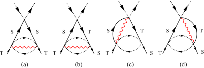
The analytical expression for diagram Fig.7.a (and similarly for b) is given by

$$\Gamma_{TT}(\omega,\epsilon)\sim(\alpha j_{2})^{2}J_{0}^{SS}T^{3}\sum_{\sigma_{1}\sigma_{2}\mu_{1}\mu_{2}}R^{\sigma\sigma_{1}\sigma_{2}\sigma}_{\mu\mu}\sum_{\epsilon_{1}\epsilon_{2}\epsilon_{3}}\sum_{\bf k_{1}k_{2}}G_{S}(\epsilon+\epsilon_{2})G_{S}(\epsilon_{2})g_{\sigma_{1}}({\bf k_{1}},\epsilon_{1})g_{\sigma_{2}}({\bf k_{2}},\epsilon_{1}+\epsilon_{3}-\omega)D(\epsilon_{3})$$

and for Fig.7.c (and similarly for d)

$$\Gamma_{TS}(\omega,\epsilon)\sim(\alpha j_{2})^{2}J_{0}^{TS}T^{3}\sum_{\sigma_{1}\sigma_{2}\mu_{1}\mu_{2}}R^{\sigma\sigma_{1}\sigma_{2}\sigma}_{\mu\mu_{1}\mu}\sum_{\epsilon_{1}\epsilon_{2}\epsilon_{3}}\sum_{\bf k_{1}k_{2}}G_{T\mu_{1}}(\epsilon+\epsilon_{2})G_{S}(\epsilon_{2})g_{\sigma_{1}}({\bf k_{1}},\epsilon_{1})g_{\sigma_{2}}({\bf k_{2}},\epsilon_{1}+\epsilon_{2}+\epsilon_{3}-\omega)D(\epsilon_{3})$$

The easiest way to calculate diagram Fig.7.a is to use the Ward Identity. The corresponding estimation is given in Section IV. As one expected, the imaginary parts of these vertex corrections have also threshold form ($|\omega|>\Delta_{ST}$).

$${\rm Im}[\rho_{0}\Gamma_{ST}^{(b)}]=\left(\alpha^{2}j_{2}^{3}\right)\left\{\begin{array}[]{ll}\displaystyle T/\Delta_{ST},~{}~{}\Delta_{ST}<T<\Delta_{ET}\\ \\ \displaystyle\omega/\Delta_{ST},~{}~{}T<\Delta_{ST}\end{array}\right.$$ (84)

The damping $\hbar/\tau$ in the frequencies interval $|\omega|<\Delta_{ST}$ is exponentially small ($\sim\exp(-\Delta_{ST}/T)$) being proportional to the population of the singlet state.

The real parts of TS vertices Fig.7.c-d are estimated as

$${\rm Re}[\rho_{0}\Gamma_{ST}(\omega,0)]\sim(\alpha^{2}j_{2}^{3})\ln\left(\frac{D}{\Delta_{ST}}\right)$$ (85)

The perturbative results including analysis of leading log and sub-leading log diagrams summarized in this section allows to incorporate noise corrections associated with the vertex fluctuator into standard one- and two- loops RG approach.

Appendix C Analytical continuation

We start with the derivation of the general equation for the vertex corrections $\Gamma_{\alpha\beta}(\omega,\epsilon)$ :

$$\Gamma_{\alpha\beta}(\omega,\epsilon)=J^{\alpha\alpha^{\prime}}J^{\alpha^{\prime}\beta^{\prime}}J^{\beta^{\prime}\beta}\int\frac{dz}{2\pi}\left[{\rm Im}G^{R}_{\alpha^{\prime}}(z)G_{\beta^{\prime}}^{R}(z+\epsilon)\Pi^{R}(\omega-z)\tanh\left(\frac{z}{2T}\right)+\right.$$

$$G^{A}_{\alpha^{\prime}}(z){\rm Im}G_{\beta^{\prime}}^{R}(z+\epsilon)\Pi^{R}(\omega-z)\tanh\left(\frac{z+\epsilon}{2T}\right)+\left.G^{R}_{\alpha^{\prime}}(z)G_{\beta^{\prime}}^{R}(z+\epsilon){\rm Im}\Pi^{R}(\omega-z)\coth\left(\frac{\omega-z}{2T}\right)\right]$$ (86)

Here the arguments in the vertex are complex variables defined in the upper half-plane,

$$\Pi(z)=\int\frac{d\epsilon}{2\pi}\coth\left(\frac{\epsilon}{2T}\right)\left[K^{R}(z-\epsilon){\rm Im}D^{R}(\epsilon)+D^{R}(z-\epsilon){\rm Im}K^{R}(\epsilon)\right].$$ (87)

Then the elastic diagonal vertex $\Gamma_{TT}$ reads

$$\Gamma_{TT}(\omega,0)=\left(J^{ST}\right)^{2}J^{SS}\int\frac{dz}{2\pi}\left[\left(G^{R}_{S}(z)\right)^{2}{\rm Im}\Pi^{R}(\omega-z)\coth\left(\frac{\omega-z}{2T}\right)+2{\rm Re}G^{R}_{S}(z){\rm Im}G_{S}^{R}(z)\Pi^{R}(\omega-z)\tanh\left(\frac{z}{2T}\right)\right]$$

This result may also be obtained by means of the Ward identity (55) for the self energy insert $\Sigma_{ST}(\omega)$ in the Green function $G_{T\mu_{1}\mu_{2}}$, which enters the triplet vertex Fig. 5.

$$\Sigma_{ST}(z)=\left(J^{ST}\right)^{2}\int\frac{d\epsilon}{2\pi}\left[{\rm Im}L^{R}(\epsilon)D^{R}(z-\epsilon)\tanh\left(\frac{\epsilon}{2T}\right)+L^{R}(z-\epsilon){\rm Im}D^{R}(\epsilon)\coth\left(\frac{\epsilon}{2T}\right)\right],$$ (88)

where

$$L^{R}(z)=\int\frac{d\epsilon}{2\pi}\left[{\rm Im}G^{R}(\epsilon)K^{R}(z-\epsilon)\tanh\left(\frac{\epsilon}{2T}\right)+G^{R}(z-\epsilon){\rm Im}K^{R}(\epsilon)\coth\left(\frac{\epsilon}{2T}\right)\right]$$ (89)

The imaginary part of Eq. (C) gives the expression (48) for the dephasing rate

No Ward identity exists for the non-diagonal vertex

$$\Gamma_{TS}(\omega,\epsilon)=\left(J^{ST}\right)^{3}\int\frac{dz}{2\pi}\left[{\rm Im}G^{R}_{S}(z)G_{T}^{R}(z+\epsilon)\Pi^{R}(\omega-z)\tanh\left(\frac{z}{2T}\right)+\right.$$

$$G^{A}_{S}(z){\rm Im}G_{T}^{R}(z+\epsilon)\Pi^{R}(\omega-z)\tanh\left(\frac{z+\epsilon}{2T}\right)+\left.G^{R}_{S}(z)G_{T}^{R}(z+\epsilon){\rm Im}\Pi^{R}(\omega-z)\coth\left(\frac{\omega-z}{2T}\right)\right]$$ (90)

References

- (1) D. Loss and D.P. DiVincenzo, Phys. Rev. A 57,120 (1998); M.A. Nielsen and I.L. Chuang, Quantum Computation and Quantum Information, (Cambridge University Press, Cambridge, 2000)
- (2) D.P. DiVincenzo, Science 720, 255 (1995); G. Burkard, D. Loss, D.P. DiVincenzo, Phys. Rev. B 59, 2070 (1999).
- (3) D. Loss and E.V. Sukhorukov, Phys. Rev, Lett. 84, 1035 (2000).
- (4) A.N. Korotkov, Phys. Rev. B 63, 115403 (2001); S. Pilgram and M. Büttiker, Phys. Rev. Lett. 89, 200401 (2002).
- (5) A. Yacoby, M. Heiblum, D. Mahalu, and H. Shtrikman, Phys. Rev. Lett. 74, 4047 (1995); A.W. Holleitner, C.R. Decker, H. Qin, K. Eberl, and R.H. Blick, Phys. Rev. Lett. 87, 256802 (2001); J. König and Y.Gefen, Phys. Rev. Lett. 86, 3855 (2001); A. Aharony, O. Entin-Wohlman, B.I. Halperin, and Y.Imry, Phys. Rev. B66, 115311 (2002); A. Aharony and O. Entin-Wohlman, Phys. Rev. B 72, 073311 (2005).
- (6) U. Gerland, J. vonDelft, T.A. Costi, and Y. Oreg, Phys. Rev, Lett. 84, 3710 (2000); Y. Ji, M. Heiblum, and H.Shtrikman, Phys. Rev, Lett. 88, 076601 (2002); A. Aharony, O. Entin-Wohlman, and Y. Imry, Phys. Rev, Lett. 90, 156802 (2002) O. Entin-Wohlman, A.Aharony and Y. Meir, Phys. Rev. B 71, 035333 (2005); T. Kuzmenko, K. Kikoin and Y. Avishai, Phys. Rev. Lett. 96, 046601 (2006).
- (7) S.A. Gurvitz, L. Fedichkin, D. Mozyrsky, and G.P. Berman, Phys. Rev. Lett. 91, 066801 (2003); A. Mitra, I. Aleiner, and A.J. Millis, Phys. Rev. B 69, 245302 (2004); J. Koch and F. von Oppen, Phys. Rev. Lett. 94, 206804 (2005).
- (8) A. Kaminski, Yu. V. Nazarov and L.I. Glazman, Phys. Rev. B 62, 8154 (2000).
- (9) J. Paaske, A. Rosch, J. Kroha, and P. Wölfle, Phys. Rev. B 70, 155301 (2004); A. Rosch, J. Paaske, J. Kroha, and P. Wölfle, J. Phys. Soc. Jpn. 74, 118 (2005).
- (10) K. Kikoin and Y. Avishai, Phys. Rev. Lett. 86, 2090 (2001); Phys. Rev. B 65, 115329 (2002).
- (11) K. Kikoin, Y. Avishai and M.N. Kiselev, Dynamical symmetries in nanophysics, arXiv-cond.mat/0407063; to be published in ”Progress in Nanotechnology Research”, Nova Science, New York.
- (12) F.D.M. Haldane, Phys. Rev. Lett. 40, 416 (1978).
- (13) C. Bruder and H. Schoeller, Phys. Rev. Lett. 72, 1076 (1994).
- (14) Y. Goldin and Y. Avishai, Phys. Rev. Lett. 81, 5394 (1998); Phys. Rev. B61, 16750 (2000).
- (15) D. Giuliano, B. Jouault, and A. Tagliacozzo, Phys. Rev. B 63, 125318 (2001)
- (16) M. Pustilnik and L.I. Glazman, Phys. Rev. Lett. 85, 2993 (2000), Phys. Rev. B 64, 045328 (2001).
- (17) M. Eto and Yu.V. Nazarov, Phys. Rev. Lett. 85, 1306 (2000), Phys. Rev. B 64, 085322 (2001); M. Eto, J. Phys. Soc. Jpn, 74, 95 (2005)
- (18) T. Kuzmenko, K. Kikoin and Y. Avishai, Phys. Rev. Lett. 89, 156602 (2002); Phys. Rev. B 69 195109 (2004).
- (19) P.W. Anderson, J. Phys. C 3, 2436 (1970).
- (20) A.S. Wightman, Il Nuovo Cimento, 110b, 751 (1995).
- (21) H.D. Zeh in Decoherence and the Appearance of a Classical World in Quantum Theory, eds. E. Joos et al (Springer-Verlag, Berlin, 2003) 2-nd ed., Chapter 9.
- (22) M.N.Kiselev, Int. J. of Mod. Phys. B, Vol. 20, 381 (2006)
- (23) M.N.Kiselev, K.Kikoin and L.W.Molenkamp, JETP Letters 77, 434-438 (2003); Phys. Rev. B 68, 155323 (2003)