Spin Precession and Real Time Dynamics in the Kondo Model: A Time-Dependent Numerical Renormalization-Group Study
Abstract
A detailed derivation of the recently proposed time-dependent numerical renormalization-group (TD-NRG) approach to nonequilibrium dynamics in quantum impurity systems is presented. We demonstrate that the method is suitable for fermionic as well as bosonic baths. A comparison with exact analytical results for the charge relaxation in the resonant-level model and for dephasing in the spin-boson model establishes the accuracy of the method. The real-time dynamics of a single spin coupled to both types of baths is investigated. We use the TD-NRG to calculate the spin relaxation and spin precession of a single Kondo impurity. The short- and long-time dynamics is studied as a function of temperature in the ferromagnetic and antiferromagnetic regimes. The short-time dynamics agrees very well with analytical results obtained at second order in the exchange coupling . In the ferromagnetic regime, the long-time spin decay is described by the scaling variable . In the antiferromagnetic regime it is governed for by the Kondo time scale . Here is the conduction-electron density of states and is the Kondo temperature. Results for spin precession are obtained by rotating the external magnetic field from the axis to the axis.
pacs:
03.65.Yz, 73.21.La, 73.63.Kv, 76.20.+qI Introduction
The decoherence and relaxation of an impurity spin is a classic problem in condensed mater physics. More then 30 years ago, Langreth and Wilkins developed a theory of spin resonance in dilute magnetic alloys. LangrethWilkins1972 The principal objective was to derive Bloch-like equations for the paramagnetic resonance using the Kadanoff-Baym KadanoffBaym62 and Keldysh Keldysh65 techniques to nonequilibrium. This included the description of spin precession and spin relaxation of a finite concentration of magnetic impurities weakly coupled to a metallic host. The recent advent of quantum-dot devices and their potential application to quantum computing has renewed interest in the spin dynamics of a single impurity. In contrast to real magnetic impurities, quantum dots can be controlled in exquisite detail, and can be tuned at will from weak coupling to the Kondo regime. Perturbative approaches, such as that of Langreth and Wilkins, LangrethWilkins1972 fail to describe the strong correlation that develop in latter regime. This calls for new theoretical approaches to nonequilibrium dynamics, suitable for treating the strongly correlated state.
In this work, we focus on the dynamics of a single spin coupled to an infinitely large environment of noninteracting particles, in order to investigate spin-relaxation phenomena at all temperatures and coupling regimes. Relaxation of a single spin is the simplest example for real-time dynamics in a quantum impurity system. Other examples might be qubits, coupled quantum dots, or biological donor-acceptor molecules. In such systems one is generically interested in the dynamics of a finite subsystem interacting with an infinitely large environment. The nature of the environment may vary from one realization to another. It can consist of a fermionic bath, as in single-electron and single-molecule transistors, or a bosonic bath, as in the spin-boson model. In certain cases a combined fermionic-bosonic bath might be in order.
The immense difficulty of treating the real-time dynamics of quantum impurity systems stems from the need to track the full time evolution of the density operator of the entire system — environment plus impurity. The Kadanoff-Baym and Keldysh techniques Keldysh65 ; KadanoffBaym62 provide an elegant platform for perturbative expansions of the density operator. In general, however, perturbative approaches are plagued by the infra-red divergences caused by degeneracies on the impurity, making them inadequate for tackling quantum impurities. Here we take an alternative approach to the real-time dynamics based on Wilson’s numerical renormalization-group (NRG) method. Wilson75
The NRG is a very powerful tool for accurately calculating equilibrium properties of arbitrarily complex quantum impurities. Originally developed for treating the single-channel Kondo Hamiltonian, Wilson75 this nonperturbative approach was successfully extended to the Anderson impurity model (symmetric KrishWilWilson80a and asymmetric KrishWilWilson80b ), the two-channel Kondo Hamiltonian, Cragg_et_al ; PangCox91 different two-impurity clusters, Jones_et_al_1987 ; Jones_et_al_1988 ; Sakai_et_al_1990 ; Sakai_et_al_1992a ; Sakai_et_al_1992b ; IJW92 and a host of related zero-dimensional problems. Recently, we extended the approach to a certain class of time-dependent problems where a sudden perturbation is applied to the impurity at time . AndersSchiller2005 Similar to the equilibrium NRG, the time-dependent NRG (TD-NRG) can be applied to all coupling strengths and is not confined to the weak-coupling regime. It is capable of accessing all time scales, including arbitrary long as well as arbitrary short times. These appealing properties make the TD-NRG a powerful new approach for studying nonequilibrium dynamics in quantum-impurity systems.
In this work, we present the complete details of the TD-NRG, and apply it to the spin dynamics of the Kondo model. A comprehensive analysis is presented for the spin relaxation and spin precession as a function of temperature, magnetic field and coupling strength. Both ferromagnetic and antiferromagnetic couplings are considered. In the Kondo regime, spin dynamics is governed by the Kondo time scale , where is the Kondo temperature of the system. In the ferromagnetic regime, the underlying time scale is strongly dependent on temperature, reflecting the fact that the effective equilibrium coupling flows to zero with decreasing temperature.
I.1 Preliminaries
The idea of applying the NRG to nonequilibrium dynamics dates back to the work of Costi. Costi97 In the spirit of the equilibrium NRG, Costi evaluated the nonequilibrium spectral functions using an individual Wilson shell for each frequency interval. However, as already recognized by Costi, Costi97 a full multiple-shell evaluation is ultimately required for the correct description of nonequilibrium dynamics. The physical reason is simple: When expanded in terms of the eigenstates of the perturbed Hamiltonian, the initial state of the unperturbed system contains contributions from all energy scales. This calls for an adequate coupling of low- and high-energy scales absent in the equilibrium NRG.
To circumvent this problem, we construct a complete basis set of the Wilson chain using the NRG eigenstates. Implementing a suitable resummation procedure, we track all states that contribute to the time evolution of the observables of interest. AndersSchiller2005 Explicitly, we have shown that the time evolution of a general local operator can be written as
| (1) |
where and are the dimension-full NRG eigen-energies of the perturbed Hamiltonian at iteration , is the matrix representation of at that iteration, and is the reduced density matrix Feynman72 in the basis of perturbed Hamiltonian. The restrictive sum over and requires that at least one of these states is discarded at iteration . In context of the equilibrium NRG, the reduced density matrix has been already used for the calculation of spectral functions. Hofstetter2000
Equation (1) is the centerpiece of the TD-NRG approach and will be heavily using throughout this paper. Below we present a detailed discussion of its derivation and implementation. Here we only wish to emphasize the following points. (i) The reduced density matrix occurs naturally in our formulation. (ii) It does not follow a unitary time evolution and, therefore, contains information on dissipation and decoherence. (iii) Equation (1) arises from summation over the complete many-body Fock space of the Wilson chain. No truncation of states is involved.
I.2 Plan of the Paper
As implied above, this paper has two main objectives: an indepth presentation of the TD-NRG and a comprehensive analysis of the spin relaxation for a single spin coupled to a conduction band. Accordingly, the remainder of the paper divides into two major parts.
The following three sections are devoted to an extensive exposition of the TD-NRG. This includes a detailed derivation of the approach, along with benchmark results for both a fermionic and a bosonic bath. Section II.2 contains a general formulation of TD-NRG for any initial density operator of the system. In particular, Eq. (1) is derived and an explicit definition of the reducted density matrix is given. In Sec. II.3, we discuss how the reduced density matrix is calculated in practice in the generic case where is the equilibrium density operator for the unperturbed system. The complete TD-NRG algorithm is outlined in turn in Sec. II.4. In sections III and IV, we compare the TD-NRG to exact results for two distinct models: the resonant-level model and a restricted version of the spin-boson model. These two test cases allow us to establish the accuracy of the TD-NRG on all time-scales, and to investigate how well a discretized finite-size system can be used to mimic nonequilibrium dynamics in a continuous bath.
Following this detailed exposition of the TD-NRG, we proceed in sections V and VI to the spin dynamics in the Kondo model. In Sec. V, we introduce the model and present some basic analytical considerations. These include an explicit calculation of the short-time response up to second order in the dimensionless exchange coupling. Numerical results for arbitrarily long time scale are covered in turn in Sec. VI, both for the ferromagnetic and antiferromagnetic regimes. Different configurations of the magnetic field are also considered. Through comparison with the analytical results of Sec. V we are able to establish the accuracy of the TD-NRG results at short time scales. The true power of the numerical solution lies, however, in the long-time behavior not accessible by perturbative techniques.
II Theoretical formulation
II.1 Goal of the method
In the present section we formulate the TD-NRG approach in general terms, before turning to concrete examples in sections III, IV, and VI. Hereafter we assume that the initial density operator at time is known, when a sudden perturbation is switch on. For , the system evolves in time with the full Hamiltonian , where is the Hamiltonian of the unperturbed system at time . Denoting the initial density operator by , the expectation value of any operator at time is given by
| (2) |
where is the corresponding time-dependent density operator.
Our first goal is to show that expectation value of any local operator can be rewritten in terms of a sum over the contributions of a sequence of reduced density matrices . Feynman72 ; AndersSchiller2005 The reduced density matrices are generated by systematically tracing out all environment degrees of freedom. Hence the unitary time evolution of the density matrix of the system as a whole is lost, giving rise to dissipation and decoherence. Although our derivation makes explicit reference to the NRG procedure, it might be applicable to other methods as well.
Two key ingredients underlie our approach: (i) The identification of a complete basis set of the many-body Fock space of the Wilson chain based on the NRG eigenstates at the different iterations; (ii) Expectation values are obtained by explicitly tracing over this complete basis set. This marks a significant departure from the conventional renormalization-group concept, where the relevant physical information is contained in the kept states. Here, the discarded states are solemnly responsible for the time evolution. This also solves the problem of overcounting excitations encountered by Costi: Costi97 Each excitation contributes only once to expectation values, at that iteration where the corresponding state is discarded. For the case where either projects onto a single state or represents the full equilibrium density operator of the unperturbed Hamiltonian, we are able give a closed analytical expression for the reduced density matrices.
II.2 Real-time evolution in quantum impurity systems
The Hamiltonian of a quantum impurity system is generally given by
| (3) |
where models the continuous bath, represents the decoupled impurity, and describes the coupling between the two subsystems. The entire system is characterized at time by an arbitrary density matrix , when a sudden, time-independent perturbation is switched on: . For , the density operator evolves according to
| (4) |
In equilibrium, one can solve such a quantum impurity system very accurately using the NRG. At the heart of this approach is a logarithmic discretization of the continuous bath, controlled by the discretization parameter . Wilson75 The continuum limit is recovered for . Using an appropriate unitary transformation, Wilson75 the Hamiltonian is mapped onto a semi-infinite chain, with the impurity coupled to the open end. The th link along the chain represents an exponentially decreasing energy scale: for a fermionic bath Wilson75 and for a bosonic bath. BullaBoson2003 Using this hierarchy of scales, the sequence of finite-size Hamiltonians for the -site chain 111We use the standard notation, by which the -site chain contains the impurity degrees of freedom, as well as the first Wilson shells (labelled by ). In contrary to the standard NRG notations we consider as dimensionfull Hamiltonian in order to emphasize the importance of all energy shells for the real time evolution. is solved iteratively, discarding the high-energy states at the conclusion of each step to maintain a manageable number of states. The reduced basis set of so obtained is expected to faithfully describe the spectrum of the full Hamiltonian on a scale of , corresponding to the temperature . Wilson75
Due to the exponential form of the Boltzmann factors, the reduced NRG basis set of is sufficient for an accurate calculation of thermodynamic quantities at temperature . This is no longer the case once the system is driven out of equilibrium. Since the nonequilibrium dynamics involves all energy scales exceeding , and in the absence of a general criterion as to which states contribute to the dynamics, a complete basis set of the Fock space of is required. In the following we identify such a complete basis set of , composed of approximate eigenstates of .
II.2.1 Complete Basis Set
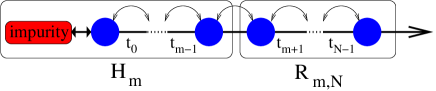
There are two possible ways to envision the iterative NRG solution of the -site chain. In the traditional picture one starts from a core cluster that consists of the impurity degrees of freedom and the site, and enlarges the chain by one site at each NRG step. Alternatively, one can view the NRG procedure as starting from the full chain of length , but with the hopping matrix elements set to zero along the chain. At each successive step another hopping matrix element is switched on, until the full Hamiltonian is recovered. In this latter picture, to be adopted below, the entire sequence of Hamiltonians with act on the Fock space of the -site chain. Accordingly, each NRG eigen-energy of has an extra degeneracy of , where is the number of distinct states at each site along the chain. The extra degeneracy stems from the “environment” sites at the end of the chain, depicted in Fig. 1.
Let us elaborate on the formal connection between the two pictures presented above. Let label the NRG eigenstates of when acting on the -site chain, and let denote their corresponding eigen-energies. Enumerating the different configurations of site by , each of the tensor-product states with arbitrary is then a degenerate eigenstate of with energy , when acting on the full -site chain. For brevity, we introduce the shorthand notation , where the “environment” variable encodes the site labels . The index is used in this notation to record where the chain is partitioned into a “subsystem” and an “environment” (see Fig. 1).
In the conventional NRG picture, the eigenstates of are constructed from the tensor-product states , corresponding to enlarging the chain by one extra site. A unitary transformation relates the new eigenstates of to the basis :
| (5) |
An alternative notation is given by
| (6) |
where the matrix elements are identified with the corresponding matrix elements of the unitary transformation : . Successively applying the recursion relation of Eq. (6), the eigenstates of can be formally viewed as matrix-product states, VmpsQIS generated by consecutive application of the matrices .
Note that the transition itself from the tensor-product states to the eigenstates involves no truncation of the Fock space. However, since the dimension of the Fock space grows as , a complete basis set is not manageable for any practical chain length of order . In the equilibrium NRG, high-energy states are thus discarded after each iteration, as these do not contribute to the equilibrium density matrix. This latter statement is guarantied by the hierarchy of scales along the Wilson chain. It would not apply to any ordinary tight-binding chain with constant hopping matrix elements.
Consider now the first iteration at which states are discarded. In order to keep track of the complete basis set of the -site chain, we formally divide the eigenstates into two distinct subsets: the discarded high-energy states and the retained low-energy states . In the course of the NRG, only the latter states are used to span the Hamiltonian within the reduced subspace . Note, however, that the sum of both subsets still constitutes a complete basis set for the -site chain. Repeating this procedure at each subsequent iteration, we recursively divide the retained subset into a discarded part and a retained part. Then, the collection of all discarded eigenstates together with the eigenstates of the final NRG iteration combine to form a complete basis set for the entire Fock space . Regarding all eigenstates of the final NRG iteration as discarded, one can formally write the Fock space of the -site chain in the form .
We stress that all states are retained in the course of this construction. Not a single state is eliminated. Since constitutes a complete basis set of , then the following completeness relation obviously holds:
| (7) |
Here the summation over starts from the first iteration at which a basis-set reduction is imposed. Typical values of are - for a spin-degenerate conduction bath. The summation indices and implicitly depend on . The identification of this complete basis set, naturally generated by the NRG, is one of the two key ingredients of our method. All traces will be carried out below with respect to this basis set. Hence, the evaluation of time-dependent expectation values involve no truncation error. Note, however, that we made no reference to a particular Hamiltonian in constructing the basis set . Below we shall make use of two distinct basis sets of this form, one for the Hamiltonian and another for the unperturbed Hamiltonian .
Another useful identity to be used below pertains to the subspace retained at iteration , . To this end, we note that the sum in Eq. (7) can always be divided into two complementary parts and :
| (8) | |||||
| (9) |
(For only exists.) The completeness relation therefore becomes
| (10) |
What do the operators and represent? The operator projects onto the subspace of all discarded states up to and including iteration . The operator projects onto the complementary subspace retained at iteration . An alternative way of writing the latter projection operator is in terms of the states retained at iteration , . Explicitly, is given by
| (11) |
II.2.2 Time-evolution of local expectation values
We are now in position to formally evaluate the time-dependent expectation value of any local operator at time . As indicated in Eq. (2), we need to explicitly carry out the trace over . This is most conveniently done using the basis set introduced in the previous section:
| (12) |
Inserting Eq. (10) in between the operators and in Eq. (12) yields
| (13) |
Using Eqs. (8) and (11) for and , respectively, we obtain , where
| (14) | |||||
and
| (15) | |||||
stem for the projection operator , and
| (16) | |||||
originates from .
Whereas the terms and involve the summation over a single iteration variable , contains two such summations: one over and another over . Rearranging the two sums according to
| (17) |
utilizing the identity
| (18) |
and replacing by the representation of Eq. (11) we obtain
| (19) | |||||
Combining Eqs. (15), (16) and (19) then yields
| (20) | |||||
Here the restricted sum implies that at least one of the states and is discarded at iteration . Terms where both states are retained contribute to the sum at some later iteration .
So far we made no assumption about the operator , nor have we committed ourselves to a particular Hamiltonian in writing the basis set . In the following we restrict ourselves to local operators . By local we mean that the operator acts on degrees of freedom that reside either on the impurity or on close-by sites for which all states are still available (i.e., ). This restriction is rather weak, since all operators in the vicinity of the impurity fulfill this requirement. The matrix elements of a local operator are diagonal in and independent of the environment degrees of freedom:
| (21) |
This allows us to write Eq. (20) in the form
| (22) |
As for the states , unless stated otherwise we work hereafter in the NRG basis set generated for the perturbed Hamiltonian . This choice is motivated by the time dependence of , which is governed by . Indeed, using Eq. (4) and resorting to the standard NRG approximation Wilson75 one has
| (23) |
Upon inserting Eq. (23) into Eq. (22), the environment variable enters only through the matrix element of . Introducing the reduced density matrix AndersSchiller2005
| (24) |
one arrives at the final result for the time evolution of at : AndersSchiller2005
| (25) |
Several comments should be made about Eq. (25). First, no assumption was made about the initial density operator . It can either project onto a particular state or represent the equilibrium density operator for . It can even stand for a density operator that has already evolved in time subject to some previous dynamics. Second, all states of the finite-size Fock space are retained in Eq. (25) and all energy scales are explicitly taken into account. No basis set reduction is imposed. This should be contrasted with recent time-dependent extensions of the density-matrix renormalization group. Marston2002 ; DaleyKollathSchollwoeckVidal2004 ; WhiteEeiguin2004 ; GobertTdDMRG2004 ; SchollwoeckDMRG2005 In the so-called TD-DMRG, the ground state is evolved in time using a Trotter decomposition of the time-evolution operator. This introduces an accumulated error that grows linearly in time. Here is evaluated independently for each time , and is thus free of accumulated errors.
This does not mean that the Eq. (25) is error-free. Two approximations enter the TD-NRG: (i) a discretized finite-size representation of the continuous bath, and (ii) the conventional NRG approximation . Indeed, the latter approximation is the only one invoked in describing the time evolution of expectation values on the -site chain. In particular, Eq. (25) is exact for . As shown by Wilson, Wilson75 the associated error in thermodynamic quantities is perturbative and small, a consequence of the separation of scales along the Wilson chain. To assess the accuracy of this approximation in the present context we have compared Eq. (25) to the exact time evolution on sufficiently short chains where all eigenstates of can be computed and stored in memory. To facilitate a meaningful comparison, only a deliberately small number of the states were kept in the course of the NRG iterations. A surprisingly good agreement was found between the exact results and the TD-NRG up to very long times, establishing the accuracy of the accepted NRG approximation in the present context.
A more significant source of error is due to the discretized finite-size representation of the continuous bath. There are two aspects to this approximation. Due to the limited energy resolution at low energies, Eq. (25) generally looses accuracy for . Since the chain length is chosen such that , one expects then a lose of accuracy for . It should be noted, however, that the NRG can access arbitrarily low temperatures, implying that arbitrarily long time scales can be reached for . We demonstrate this important point later on. At the same time, a continuous spectrum is expected to be vital for relaxation to the exact thermodynamic expectation value with respect to . This constitutes a fundamental obstacle for any solution, however accurate, of a finite-size system. As detailed in subsection II.5, we can largely overcome this obstacle by (i) averaging over different realizations of the Wilson chain using Oliveira’s -trick, YoshidaWithakerOliveira1990 and (ii) resorting to a Lorentzian broadening of the NRG levels.
II.3 Calculation of the reduced density matrix
So far, our discussion applied to a general local operator and to an arbitrary initial density operator . The time evolution of was shown to be determined by a sequence of reduced density matrices , in which the environment degrees of freedom are traced out iteratively. While formally applicable to any , practical calculations may prove more restrictive. Here we address the calculation of the reduced density matrix.
Typically, has a simple representation with respect to the eigenstates of the unperturbed Hamiltonian . For example, starting from thermal equilibrium is equal to , where is the unperturbed partition function. Thus, the reduced density matrix is most conveniently expressed with respect to the NRG eigenstates of the unperturbed Hamiltonian, i.e., when the states in Eq. (24) relate to . Note, however, that the reduced density matrix which enters Eq. (25) was explicitly constructed for the NRG eigenstates of the full Hamiltonian . In general, there is no simple relation between the two reduced density matrices, as they involve traces over different environments. Still, one can convert between the two entities in the generic case where the system is evolved in time from thermal equilibrium. Below we explain in detail how the reduced density matrix of Eq. (24) is calculated for this generic case.
II.3.1 General considerations
Let us assume for the time being that the reduced density matrix is know with respect to the NRG eigenstates of the unperturbed Hamiltonian . Namely, when the states that enter Eq. (24) correspond to . Our goal is to compute the reduced density matrix with respect to the NRG eigenstates of the full Hamiltonian . Technically, this requires working with two distinct sets of NRG states — one for and the other for . To simplify the notation as much as possible, we distinguish the two sets of states by their labels. Throughout this subsection we designate the NRG states pertaining to the unperturbed Hamiltonian by indices carrying the subscript . For example, the state . NRG states corresponding to will be labeled, as before, with plain indices having no additional subscripts as in . We stress that and label the same environment degrees of freedom, despite the difference in appearance. Similarly, we reserve the notation for the reduced density matrix as defined in Eq. (24) with respect to the states of the full Hamiltonian . The reduced density matrix with respect to the states of the unperturbed Hamiltonian is denoted (and defined) by
| (26) |
As shown in the previous subsection, one can write the completeness relation for any Hamiltonian . The projection operators and are simply written in this case using the NRG states of [see Eqs. (8) and (11)]. Below we apply this completeness relation for the initial Hamiltonian , with one slight modification. Shifting the term from Eq. (8) to Eq. (11) one has the identity
| (27) |
where
| (28) |
and
| (29) |
Here the index in Eq. (29) runs over all NRG eigenstates of iteration , whether discarded or retained. This shift of notation from to is of purely practical nature as it allows us to sum freely over all states of any given iteration . The symbol is used to emphasize the different complete basis sets of and .
We are now in position to address the reduced density matrix . Starting from Eq. (24), we make use of the completeness relation of Eq. (27) in order to replace with
| (30) |
Equation (24) is decomposed in this fashion into four contributions:
| (31) |
where equals
| (32) |
(). Of these four components, only can be directly related to the “unperturbed” reduced density matrix of Eq. (26). To see this, we insert Eq. (29) into Eq. (32) to obtain
| (33) | |||||
This expression features the overlap matrix elements , which are diagonal in and independent of the environment degrees of freedom:
| (34) |
The reduced matrix records the overlap matrix elements between the NRG eigenstates of and . It is conveniently computed in the course of the NRG iterations as described in Appendix A. With the matrix at hand, is obtained by a simple rotation of the “unperturbed” reduced density matrix into the new basis:
| (35) |
Note, however, that this transformation is not unitary due to basis set reduction at each iteration. Hence, follows directly from the knowledge of .
In contrast to , the remaining components , and cannot be related in any simple way to the “unperturbed” density matrix . This is readily seen by inserting Eq. (28) into Eq. (32), which gives rise to overlap matrix elements of the form with . The latter matrix elements generally depend on both and , which prevents from collapsing the trace over to the form that appears in Eq. (26). At present we have no feasible way to carry out such a trace.
Physically, the terms , and encode the way in which high- and low-energy eigenstates of are coupled within . For these terms to be important, must contain a significant contribution from high-energy states, which means starting from a state well removed from thermal equilibrium. In the following we restrict attention to the case where corresponds to thermal equilibrium, or more generally to the case where .
(a) 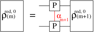
(b) 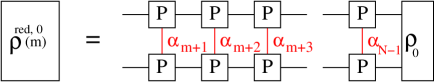
II.3.2 Starting from thermal equilibrium
Upon starting from thermal equilibrium, takes the standard form , where is the unperturbed partition function. In terms of the appropriate NRG basis, it has the spectral representation Wilson75
| (36) |
| (37) |
These expressions neglect all states discarded at iterations , exploiting the fact that the discarded states have only an exponentially small contribution to at the temperature . Wilson75 This NRG approximation usually works very well, and can be systematically improved by increasing the number of states retained at the conclusion of each NRG iteration. We denote the latter number of states by .
By construction, Eq. (36) obeys the operator identity . This guarantees that , and identically vanish for all . Hence is fully determined by according to Eq. (35). We now elaborate how is computed recursively from . Together with the “initial” condition
| (38) |
this provides us with for all .
Consider an arbitrary . To execute the sum over in Eq. (26), we set , where encodes the site labels . In other words, is a state variable for the environment , see Fig. 1. Substituting in for , and using the overlap matrix elements
| (39) |
[see Eq. (6)], Eq. (26) is expressed as
| (40) | |||||
where the sum over and is restricted to the states retained at iteration . (For , the sum runs over all the states of the final NRG iteration). In the standard case of a real Hamiltonian , the matrix elements are likewise real. Under these circumstances one can omit the complex conjugate from . It is also easy to verify that vanishes if at least one of the states and is discarded at iteration . This is a simple consequence of the orthogonality of our basis-set states and the spectral representation (36), i.e. , for all . The recursion relation can also be visualized diagrammatically depicted in Fig. 2 as brought to our attention by Weichselbaum.
Note that the recursion relation of Eq. (40) is not confined to thermal equilibrium. It relied solely on the fact that , which guaranteed that for all . No additional restriction was made to an equilibrium distribution. Nevertheless, one is typically interested in the case where the system starts from thermal equilibrium. The “unperturbed” reduced density matrix coincides then with the one originally introduced by Hofstetter for the purpose of calculating equilibrium spectral functions within the NRG. Hofstetter2000
II.4 TD-NRG algorithm
After the exposition of the different components of the TD-NRG approach, we now turn to the integrated algorithm. To implement the TD-NRG at temperature , one first selects a chain length such that . Two simultaneous NRG runs are then performed, one for and another for . All NRG eigen-energies of and are stored up to the final iteration . At each iteration , the overlap matrix of Eq. (34) is calculated between all eigenstates and of and , respectively. Details of the calculation are elaborated in Appendix A. This information, as well as the product matrices for the initial and final Hamiltonian, are stored on the hard drive. After the final NRG run, the equilibrium density matrix is calculated from Eq. (36) using the eigenstates and eigen-energies of last NRG iteration for .
At the conclusion of these steps, the TD-NRG proceeds by backward iterations starting from . For each backward iteration from to , the following three steps are performed:
-
1.
The “unperturbed” density matrix is calculated from using the product matrices for the initial Hamiltonian , in combination with the recursion relation of Eq. (40).
-
2.
The reduced density matrix is computed by rotating to the basis of the final Hamiltonian using the overlap matrix and Eq. (35).
-
3.
Using Eq. (25), the contribution of iteration to is evaluated simultaneously for all times of interest. Here the only matrix elements of and to contribute are those where at least one of the states and is discarded at iteration . At the conclusion of this step, is deleted to reduce the memory load.
These steps are repeated until is reached, below which no state has been discarded.
It is easy to see that if , i.e., the Hamiltonian is left unchanged, then so obtained coincides with the thermodynamic average of for all . Indeed, the overlap matrix is diagonal in this case, which means that and are the same. Consequently, has nonzero matrix elements only if the states and are both retained, leaving only the iteration to contribute to Eq. (25). Since coincides with the equilibrium density matrix which is diagonal in energy, one recovers the thermodynamic average of independent of .
A word is in order at this point about the nonequilibrium NRG approach of Costi, Costi97 and its relation to the TD-NRG. Costi had focused on the calculation of nonequilibrium spectral functions. In contrast to the TD-NRG, he settled with a single NRG shell to evaluate the spectral function at frequency . In practice this meant replacing the reduced density matrix with the full equilibrium density matrix at iteration . After rotating the latter according to Eq. (35), only a single Wilson shell contributes to a given of the spectral representation of . Being well aware that a full multiple-shell evaluation is ultimately required for the correct description of nonequilibrium dynamics, Costi97 Costi carefully applied the single-shell approach only to intermediate frequencies. This restricted his ability to track the real-time dependence of .
In the TD-NRG we overcame these difficulties by identifying an appropriate basis set for the Hilbert space of the -site chain, and by the resummation procedure that has led to Eq. (25). The significance of these steps is best reflected in the fact that of Eq. (25) exactly coincides for any local operator with its NRG thermodynamic average with respect to . While physically clear, this statement is highly nontrivial from the standpoint of the TD-NRG, as all energy scales contribute to the summation of Eq. (25). Moreover, the limit stems from the degenerate terms with from all iterations in Eq. (25). In frequency domain, these terms give rise to an addition contribution that comes out naturally in the TD-NRG, but is absent in Costi’s approach. The latter is of crucial importance for obtaining the correct asymptotic long-time behavior of operators with non-vanishing expectation values.
II.5 Towards restoring the continuum limit
So far, we focused on accurately calculating the time evolution of any local observable on a finite-length chain. While this might be a reasonable representation of mesoscopic systems characterized by a finite level spacing, our approach is geared toward the description of a continuous bath. Relaxation in such a macroscopically large system cannot be fully described by a finite Wilson chain. Indeed, it was already pointed out in the context of the equilibrium NRG YoshidaWithakerOliveira1990 that certain thermodynamical properties undergo unphysical oscillations as a result of the discretization of the continuous bath. To circumvent this problem, Oliveira and coworkers YoshidaWithakerOliveira1990 introduced a -dependent logarithmic discretization of the continuous bath according to . Wilson’s original discretization corresponds in this notion to . As shown by Oliveira et al., the unphysical oscillations can be removed by integrating expectation values with respect to . This has the effect of mimicking a continuous bath using a single adjustable parameter.
We apply the same technique to improve on the computation of time-dependent quantities. To partially mimic the relaxation in an infinite-size system, we calculate the time evolution of Eq. (25) for each value of , , and average over the different ’s. Here is the total number of -values considered. Since the NRG oscillations are primarily associated with and terms on the interval , YoshidaWithakerOliveira1990 should be chosen in multiples of . This leads to optimal cancellation of oscillations. As shown below (see Fig. 3), usage of the -trick can greatly improve on the long-time behavior of the TD-NRG.
Even with the -trick at hand, the evaluation of boils down to summation over a finite number of oscillatory terms of the form . One way to simulate a continuous spectrum is to broaden the NRG levels, as is done in the calculation of equilibrium spectral functions. This requires, however, extra care in the nonequilibrium case. As mentioned above, the limit originates from the time-independent terms with in Eq. (25). These terms must remain in tact in order to correctly describe the long-time behavior. Therefore, one must separate the time-independent terms from the oscillatory ones. Damping should only enter the latter terms in Eq. (25).
Focusing on the oscillatory terms, we replace each energy with a Lorentzian broadening according to
| (41) |
Here with a constant of order one is a scale-dependent broadening, reflecting the characteristic energy resolution of the th NRG iteration. In this fashion, each of the terms in Eq. (25) is modified according to
| (42) |
while the terms with are left in tact. Below we present results with and without the additional damping factor .
It should be noted that the Lorentzian broadening of Eq. (41) differs from the customary log-normal form used for equilibrium spectral functions. This choice is motivated by physical considerations, as it produces a simple exponential decay in time. We also stress that comes to simulate the continuous spectrum of the bath. Should possess eigenstates which are pure eigenstates of the impurity part of the Hamiltonian and do not couple to the bath (as is the case in certain parameter regimes of electron-transfer models TornowBulla2005 ), must be set to zero. Else, unphysical damping is introduced.
II.6 Discussion of the TD-NRG approach
For clarity, we summarize the key ingredients as well as the assumptions made in the TD-NRG approach in this section. We have to divide the different aspects of conceptual and technical nature.
As mentioned in the previous section, one of the most important conceptual points to bear in mind is the mimicking of a continuum of bath degrees of freedom by a selection of discrete states. Therefore, we expect always some oscillatory contributions in the time evolution of : the shorter the chain length, the smaller the amount of bath degrees of freedom the stronger the oscillations. This property is inherent to any discrete representation of a continuum and not a shortcoming specific to our method. In fact, the mapping error is controlled by the NRG discretization parameter and the chain length becomes infinite for a given temperature for . In addition, we could show that these oscillations are strongly suppressed by the -trick described in the previous section also mimicking a bath continuum.
Another conceptual point concerns our expectation of the time evolution. If we would include all possible physical interactions, have all baths for energy and particle exchange coupled to the system, wait an infinitely amount of time, we expect that the system equilibrates to the new thermodynamic equilibrium governed by independent of the initial conditions. This is required by the basic assumption of equilibrium thermodynamics. However, this is in general not the case. Imagine an isolated spin in metallic host in strong magnetic field, as we will investigate later in the section on the Kondo model. If we artificially decouple this spin from the environment and switch of the external magnetic field, the local spin will remain its polarized steady state rather than relaxing to the new thermodynamics state since the local spin remains a conserved quantity. The local expectation value can only evolve towards the new thermodynamics equilibrium, if provides an energy, magnetization or particle exchange mechanism.
Imagine, is controlled by an external time-dependent field which couples to a conserved quantity of the total system, i. e. and . Then all eigenstates of remain eigenstates to for arbitrary times. Only the eigen-energies obtain a time-dependent shift , where is the eigenvalue of of state . It is obvious that there will be no time dependence of any operator whose matrix elements are energy-independent such as spin or charge.
Another non-trivial difference to the assumption of thermodynamics arises from the fact that we describe the time-evolution of a closed system. This is in contrast to the Keldysh approach Keldysh65 which introduces - usually in a very subtle - an infinitely small relaxation rate much smaller than any energy scale in the problem to ensure the asymptotic approach of the thermodynamical state. Sometimes, even explicitly the existence of an additional thermodynamic bath is made. In our description, however, the total energy of the system remains a constant and is given by
| (43) |
since the time evolution operator commutes with . In contrary, the total energy of the thermodynamical equilibrium is given by
| (44) |
where . A sudden change in the Hamiltonian of closed finite size system will always result in an effective heating, where the effective temperature can be obtained by solving the implicitly equation
| (45) |
If the energy of the bath states of , however, are continuously distributed and their energies are not changed by , the temperature will not be changed in the thermodynamic limit.
III Fermionic benchmark: Resonant level model
III.1 Definition of the model
The resonant-level model is perhaps the simplest example for a quantum-impurity system. A single Fermionic level with energy is coupled by hybridization to a bath of spinless Fermions:
| (46) | |||||
Here creates an electron with momentum in an s-wave state about the position of the level (taken to be the origin). To make connection to the TD-NRG approach, we consider a step-like change in and : and . Since the model is bilinear in Fermionic operators, equilibrium properties (i.e., for and ) can be calculated exactly using, for instance, the local Green function :
| (47) |
| (48) |
In the wide-band limit, defines the width of the level due to the coupling to the Fermionic bath.
III.2 Analytical Keldysh solution for nonequilibrium
Out of equilibrium, the occupancy of the level, , follows directly from the knowledge of the equal-time lesser Green function . Using the Keldysh technique, Keldysh65 ; LangrethWilkins1972 we derived an exact analytical expression for in the wide-band limit, for a step-like change of parameters at :
| (49) |
with
| (50) | |||||
Here, is the density of states of the Fermionic bath, is the Fermi-Dirac distribution function, equals , and ().
Besides the wide-band limit, Eqs. (49) and (50) require that , which comes to ensure that the initially decoupled level for has decayed to its equilibrium state for . Since any infinitesimal value of fulfills this requirement, the limit can be viewed as contained in Eqs. (49) and (50).
For , Eqs. (49) and (50) can be evaluated in closed analytic form. Introducing the auxiliary function
| (51) | |||||
where is the exponential integral function, we obtain
| (52) | |||||
Here with is the equilibrium occupancy of the level for the corresponding model parameters, and .
We note that the exact result does not exhibit a simple exponential decay to the new equilibrium occupancy . It is actually governed by two relaxation rates, and . Moreover, the last and second-to-last terms in Eq. (52) contain an oscillatory factor , responsible for Rabbi-type oscillations that visible for at short time scales. In a previous publication, AndersSchiller2005 we have used this rather elaborate formula and its extension to finite temperatures to benchmark the TD-NRG. Here we complete the discussion by focusing on the role of the NRG parameters and .
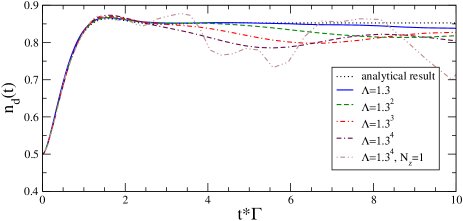
Figure 3 presents a comparison between the exact analytic result of Eq. (52) and the time-dependent occupancy obtained by the TD-NRG for different values of and . The temperature is roughly kept fixed in all curves by adjusting the length of the NRG chain. While the curve corresponding to the smallest value of and, thus, to the longest chain used () shows excellent agreement with the exact analytical result on all time scales, the curves for the larger values of show good agreement only at shorter times, . Deviations from the exact result develop at longer times, which are characterized by oscillations about a value of that is reduced as compared to the new thermodynamic average. We emphasize that none of the TD-NRG curves in Fig. 3 involved an extra damping factor .
The above behavior is not surprising since, as discussed in Sec. II.6, the shorter the NRG chain, the worse it represents a continuous bath. A different way of viewing the matter is through the conservation of energy and particles in the system for . In a macroscopic bath, the system relaxes to the new equilibrium state by redistributing the excess particles among the different lattice sites. Since the excess number of particles is of order one, each lattice site (the level included) acquires an infinitesimal shift to its occupancy, which vanishes in the thermodynamic limit. For a finite system, the shift in occupancy remains finite. We therefore conclude that the oscillations depicted in Fig. 3 are real in a finite-size system. However, they are unphysical for a continuous bath, as demonstrated by the exact analytical solution. We pinpoint this “inaccuracy” to be of conceptual nature, controllable by the limit .
The magnitude of the finite-size oscillations is greatly reduced, though, by resorting to Oliveira’s z-trick. To illustrate this point, we have added one extra curve for without any -averaging. Enhanced by the short chain length, the finite-size features are notably more noisy and have a larger amplitude. The effect of averaging over is to greatly smoothing and reduce these finite-size structures. Hence averaging over is vital for describing the long-time behavior, particularly if no extra damping is introduced.
The short time behavior, however, is very accurately reproduced defying prejudice against the NRG which allegedly is insufficient to describe the high energy physics correctly needed for the short time behavior. Even if the statement would be true, the NRG represents the high energy physics incorrectly for calculating thermodynamics properties, which is not – see Wilson Wilson75 – it would have no influence on the time evolution calculated with the TD-NRG for a very simple reason. The high energy states are generated at the first iterations. For energy scales much larger than the relevant scales of the quantum impurity, the NRG flow of and are more or less identical which leads to a almost diagonal overlap matrix for these iterations. Since the reduced density matrix is only non-zero for retained states there will be no contribution to the time evolution when evaluating (25). Only when the flow between the two Hamiltonians starts to deviate, contributions to the expectation value are generated. This may be seen clearly in the inset of figure 2a of our previous paper AndersSchiller2005 which shows the iteration dependent evolution of .
IV Bosonic benchmark: decoherence in the spin-boson model
The spin-boson model Leggett1987 ; Weiss1999
| (53) | |||||
is perceived as the simplest model for the understanding of dissipation and decoherence in quantum systems. A two-level system, represented by a spin, is coupled to the displacement operator of a continuum of bosonic degrees of freedom with the coupling constant to each bosonic mode. This continuum causes decoherence, dissipation and possible spin decay. The effect of this dissipative environment is fully captured by the coupling function
| (54) |
Since the low-energy part of the spectrum dominates the response of the spin, the high-energy details of can be neglected: this function is usually approximated by a power-law behavior Leggett1987 : , . In the literature, one distinguishes between the “ohmic” case, , corresponding to a classical model with a dissipative term proportional to the velocity, the “sub-ohmic” case and the “super-ohmic” case . In the ohmic regime, the spin-boson model can be mapped onto the anisotropic Kondo model in the wide-band limit, Leggett1987 with and .
This model plays also an important role for understanding charge transfer reactions in chemistry XuSchulten1994 where the spin states would represent the initial and final state of the transfer reaction and the bosonic continuum the density fluctuations of solvents or molecular vibrations. It has been argued XuSchulten1994 ; Schulten2000 that the model serves a quantum mechanical foundation of the classical Marcus theory Marcus1993 for electron transfer reaction.
In addition, the model has been discussed in the context of decoherence of qubits in quantum computing Unruh1995 ; PalmaSuominenEkert1996 . Setting , is a conserved quantity, and, therefore, the bosonic environment can be traced out analytically. If we prepare an initial density matrix containing locally only the pure state , it was shown PalmaSuominenEkert1996 that off-diagonal part of the reduced density matrix
| (55) |
can be written as . Here, is given by the exact expression
| (56) |
for the temperature . Unruh1995 ; PalmaSuominenEkert1996
Recently, Bulla and collaborators introduced an extension of the NRG to bosonic baths.BullaBoson2003 ; BullaVoita2005 These authors investigated the different quantum critical points of the model as a function of the bath exponent and the coupling strength . We combined their bosonic NRG method and our TD-NRG approach to show explicitly that our method is very accurate for short as well as long times up to for bosonic baths as well.
In order to start with the same boundary conditions as the exact result was derived for, we set in . This guarantees that equilibrium density operator consists of the disentangled operator product of and the equilibrium density matrix of the bosonic bath for . For , is set to zero and an entangled density matrix is evolving with time. The off-diagonal matrix element corresponds to the expectation value of obtained by the bosonic TD-NRG. The coupling function
| (57) |
enters the analytical as well as the numerical calculation. We have obtained for fixed and different exponents . The comparison between the TD-NRG and the exact analytical result given by Eq. (55) is depicted in Fig. 4 for the super-ohmic, the ohmic and the sub-ohmic case. We observe excellent agreement between the exact analytical result and the predictions of the TD-NRG. 222A detailed analysis of the dynamical properties of spin-boson model will be published elsewhere. The small oscillations in the quantum regime observed in all curves in the time range are no artifacts of the method but real features. By comparison with the exact analytical result, they have been traced to the usage of the hard frequency cutoff in at . Using a soft cutoff function would produces smoother and slightly shifted curves.PalmaSuominenEkert1996
We noted that due to the larger numbers of degrees of freedom added though each chain link, the time evolution for a bosonic bath shows a higher accuracy and less dependence on than for fermionic baths as long as one does not leave the range of validity of the bosonic chain NRG. BullaVoita2005
V The Kondo model: analytical considerations
V.1 Definition of the model
The Kondo model comprises of a local spin interacting with a spin degenerate conduction band via a local anisotropic Heisenberg term
where creates a conduction electron at the position of the spin . For , we obtain the usual symmetric interaction. We also allow for a time-dependency of the coupling constants and . The energy of the local levels are splitted in an external magnetic field by the Zeeman energy
| (59) |
whose transversal parts can also be interpreted as hopping terms of the two-level system modelled by the local spin 1/2. The local conduction electron creation operators are expanded in s-wave eigenmodes of the non-interacting conduction electron band
| (60) |
where denotes the conduction electron density of states. 333Even though the formulation is quite general, we will use a constant density of states and a symmetric band for all numerical calculations throughout the paper. Note that the anti-commutator of the local conduction electron operator is given by . The conduction electron Hamiltonian is given by
| (61) |
where creates (annihilates) electron in an s-wave state with spin , energy . All other angular momentum do not interact with the local spin.Wilson75 The integration runs from the lower to the upper band edge, to . Throughout the paper, we assume a symmetric band with a relativistic dispersion, i. e. and . Then, the total Hamiltonian under consideration is given by
| (62) |
Why do we neglect the spin polarization of the conduction electrons? As we discussed in section II.6, an external field coupling to total -component of the spin yields a time independent local spin expectation. Since the external magnetic field, however, couples to the total magnetization
| (63) | |||||
where is the local spin operator and the total spin of the conduction electrons, the relevant Zeeman energy for the real time dynamics is given by . In this case, the local spin can relax if the gyromagnetic ratios of local spin and conduction electrons differ. Then, would have to be replace by in Eq. (59).
In real materials, however, the spin-orbit scattering of the conduction electrons on distributed impurities in the metallic host furbishes another relaxation mechanism, as pointed out by Langreth and Wilkins LangrethWilkins1972 more than 30 years ago. We might argue in the following way. If this relaxation processes for the conduction electron magnetization is much faster than the relaxation process of the impurity spin due to coupling to the conduction electrons, we can consider the conduction electron band as demagnetized on the time scale of the impurity relaxation process. In this case, neglecting the spin-polarization of the conduction electrons are justified. If for some reason, the spin-lattice relaxation processes is very slow compared to the impurity spin, the impurity spin-relaxation process is dominated by the spin-lattice relaxation time in which case we have to substituted or rescale the absolute values of the physical magnetic field.
It turns out, that the long-time behavior of impurity spin relaxation is dominated by the Kondo time in the Kondo regime, given by the reciprocal characteristic thermodynamic energy scale , and by the reciprocal temperature for the ferromagnetic regime of the model. As long as the spin-lattice relaxation time is finite, for sufficiently low temperature and Kondo temperature , neglect of the conduction electron spin-polarization is justified. However, the short time behavior of the spin relaxation has admittedly purely academical value if .
We will distinguish between two different starting positions. Either we leave the coupling constant unaltered and just switch of the magnetic field at , which is the physically more relevant condition. Alternatively, we start from an initially decoupled system, the local moment fixed point of the Hamiltonian, and switch on the Kondo couplings and as well as changing the applied magnetic field at time . It was previously pointed out NordlanderEtAll1999 ; AndersSchiller2005 that this setup is closer to the thermodynamics since the time might play a similar role as .
V.2 Analytical results
Wilson invented the numerical renormalization groupWilson75 to solve the thermodynamics of this model very accurately for all parameter regimes. The model has two fixed points for the antiferromagnetic regime, the unstable local moment fixed point corresponding to and the stable strong coupling fixed point for caused by the infrared divergence in the perturbation theory in the absence of an external magnetic field. For the ferromagnetic regime, i.e. and , the stable fixed point is given by . Due to the ferromagnetic polarization of the conduction band in the vicinity of the impurity, the spin-flip scattering is more and more suppressed for decreasing temperature: the model remains perturbative in this regime.
The analytical “poor man’s scaling” second-order renormalization group treatmentAnderson70 prior to the NRG predicts
| (64) |
The renormalization of isotropic coupling as of the running cutoff
| (65) |
provides some analytical inside for the fixed point structure even though the treatment breaks down for .
For the isotropic ferromagnetic Kondo model, however, remains finite and vanishes for . Since the model approaches the local moment fixed point in this case, a spin-polarized local state remains spin-polarized after switching of the magnetic field at without any additional relaxation mechanism present. At finite temperature, however, a thermal energy of provided fluctuations in the bath in addition to the very small but finite transversal spin flip term . Therefore, we expect that the FM Kondo model has a characteristic time scale which is actually found in the calculations (). Through the paper we measure the temperature in energy units (.)
V.3 Short time behavior and relaxation towards the Kondo strong coupling fixed point
If we consider a decoupled impurity for times , we can calculate analytically the short time response using a perturbation expansion. For and , the equilibrium density operator is given by where . Switching on the coupling , at leads to the time evolution of spin operator
| (66) |
where , if the magnetic field is switched off for . In the interaction picture, the spin operator
| (67) |
obeys the equation of motion
| (68) |
which is integrated to
where . Neglecting the last term yields a perturbative result correct up to order . Since commutes with the term in , its short time behavior is solemnly governed by . The renormalization of by sets in at third order, well known for the Kondo problem. Hewson93 Alternatively, the time evolution of could have also been calculated using Keldysh techniques.LangrethWilkins1972 All expectation values have to be evaluated with equilibrium density operator . Since we are only interest in an analytical results for short times, the Keldysh approach does not have any advantages: it also fails to capture the Kondo physics at long time scales.LangrethWilkins1972
There will be no contribution linear in since . Evaluation of the two commutators needed for the second order contribution in (V.3) yields
| (70) | |||||
For and a constant density of states , we can solve the integrals analytically and obtain
where we have defined the function by its series expansion
| (72) |
The result is exact up to : the short time evolution is independent of , consistent with the physical picture that a change of the spin state can only by mediated by the spin-flip term of Kondo interaction. enters at first in the third order of the perturbation expansion, corrections which are neglected here.
VI The Kondo model: numerical results of the TD-NRG
VI.1 Antiferromagnetic regime
VI.1.1 Short and long time behavior for
In order to make connection between the TD-NRG and the analytical calculation for the short time behavior presented in previous section, we start with a decoupled impurity in a finite magnetic field along the z-axis, i.e. . At , we switch on the anisotropic Kondo interaction and simultaneously switch off the magnetic field. At infinitely long times, we expect that the system will relax into the strong coupling Kondo fixed point for and , independently of the initial conditions.
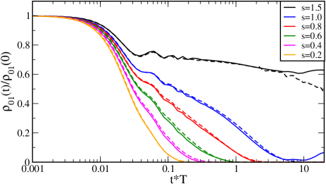
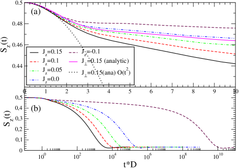
In Fig. 5, the time evolution of is shown for a fixed spin flip rate and different values of . is independent of as expected for times , clearly visible in the upper panel (a). Only spin-flip processes can alter the spin polarization. At short times, the Kondo correlations are absent. Only the bare coupling constants enter the analytical result calculated for the comparison with the presented TD-NRG curves. The magenta (online) curve in (a) displays the second contribution in given by Eq. (V.3) which contains arbitrary high orders in through the series expansion of .Since the analytical formula is independent of , it must correspond to the TD-NRG curve for . We find an excellent agreement between the analytical and the TD-NRG result confirming the accuracy of our method at short and intermediate time scales. These findings show that the ultra-short time response is purely perturbative, since the strong correlations develop only at low energies and, therefore, influence only the long time behavior. The curves lie below, the curve with a ferromagnetic above the analytical results. Starting with order , terms contribute to by renormalizing . The positive leads to an increase of , while a ferromagnetic yields a reduction of consistent with our findings in Fig. 5a) of an increasing relaxation time scale with decreasing . The long-time behavior of is displayed in Fig. 5b). Note that the TD-NRG accurately predicts the relevant time scales of the spin relaxation for arbitrary long time scales, here over 10 orders of magnitude in units of the reciprocal band width as long as .
| 0.15 | 0.000537 | 1862.3 |
|---|---|---|
| 0.10 | 0.000203941 | 4903.4 |
| 0.05 | 18211 | |
| 0.0 | 124850 | |
| -0.1 |
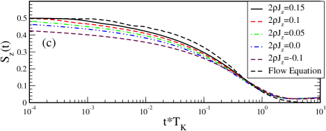
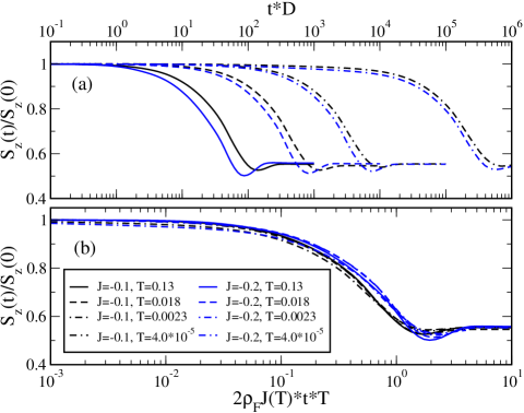
In order to identify the long time scale, we rescale the data with the thermodynamic Kondo temperature which is obtained from the temperature dependency of the effective local moment Wilson75 . Excellent scaling is found for the long time tails. Instead of using the thermodynamic Kondo temperature, we could have defined an effective time scale by which is reduced to 20% of the starting value . It turns out that independent for within the numerical accuracy. Therefore, the two time scales are equivalent, and the Kondo time governs the long time behavior of .
From this discussion, it is apparent that there will be no universal master curve for valid for all times and solemnly parametrized by a universal time scale . Only at very long times , the curves tent to approach a universal curve . The panel (c) of Fig. 5 presents how the value of determines this approach to this master curve. We also added the universal curve for the weak coupling isotropic Kondo model, i.e. . Lobaskin and Kehrein have calculated this curveLobaskinKehrein2005 using Wegner’s flow equation Wegner1994 and expanding the solution at the exactly solvable Toulouse point. The quantitative agreement between their result and the TD-NRG for isotropic Kondo model is very good. However, our calculations also show that the transients towards the ultra long time behavior at time scale are still dependent of the anisotropy ratio . Deviations from lead to deviations from an master curve for an isotropic Kondo model. Only at , we expect the merging of the curves.
VI.1.2 Finite temperature relaxation
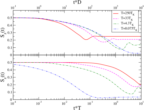
Starting from a decoupled, fully spin-polarized impurity, the temperature dependence of the spin relaxation is plotted in Fig. 6 for the isotropic, antiferromagnetic Kondo spin. The characteristic spin-relaxation time saturates for temperatures and is of the order of at very low temperatures, similar to the findings in the single impurity Anderson model. AndersSchiller2005 The upraise of for very long times at the temperatures is an artifact of the insufficient time resolution at high temperatures. To illustrate this point, the same data is plotted as function of in the lower panel (b).
VI.1.3 Magnetic field dependence of the spin relaxation
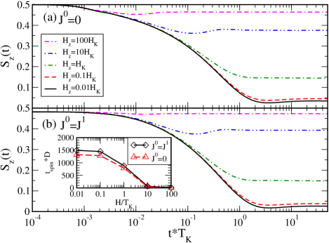
The time evolution of a polarized decoupled Kondo spin with Hamiltonian with a remaining finite local magnetic field is plotted in Fig. 7. For the local spin is fully polarized by a strong magnetic field. The figure shows the evolution of for five different magnetic field strength , where the Kondo scale is given by for . For the upper panel (a), the local spin was decoupled from the bath for times , while the curve in the lower panel (b) were calculated for a Kondo spin coupled to the bath at all times. The difference in the time evolution between the two scenarios are very small in contrary to our previous study of the single impurity Anderson model AndersSchiller2005 . The strong magnetic field destroys the Kondo correlation and the regimes are described by a spin polarized local moment fixed point in both cases: the Kondo spin-flip scattering is an irrelevant operator due to the external field. In the Anderson model, however, the fixed points of both scenarios are completely different: in case of an absent hybridization, we have a free orbital or local moment fixed point while for finite coupling we started from a spin polarized mixed valent fixed point.
Fig. 7 clearly shows a decrease of the characteristic time scale with increasing final magnetic field. In order to quantify this behavior, we asked how long does it take until the spin-expectation value reaches some fraction of its asymptotic value . For this purpose, we introduce the reduced spin expectation value function
| (73) |
and define a magnetic field dependent spin-relaxation time scale by the condition: . Note that the time scale does not have the meaning of a reciprocal relaxation rate, since is – in general – not an exponential function. The choice of generalizes the criterion given for at the end of section VI.1.1. While the value is arbitrary, of course, but setting to or yields the same qualitative picture as depicted in the inset of Fig. 7b). For very weak magnetic fields, , the spin-relaxation time remains almost field independent while for the relaxation time rapidly drops and reaches for (a) and at .
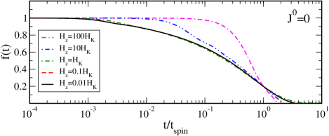
In order to demonstrate the usefulness of the scale , we rescale the data of Fig. 7a) in dimensionless units using Eq. (73) and plot the resulting versus the dimensionless time scale . The result is depicted in Fig. 8. For magnetic fields much larger than the Kondo temperature , the spin relaxation is “fast” since the asymptotic value is reached rather rapidly. No Kondo correlations develop and no universality is observed. For , however, all curves collapse onto a universal curve as clearly visible in Fig. 8.
VI.2 The ferromagnetic regime
VI.2.1 Short and Long time Behavior
As discussed in section V.2, the ferromagnetic regime of the Kondo model is governed by the vanishing of for . For the isotropic Kondo model, the Hamiltonian flows towards the local moment fixed point. Anderson70 ; Wilson75
We start with a Kondo spin, always coupled to the bath, i.e. and only subject to a switched magnetic field. In this case, the strong correlations already form at times . In Fig. 9a), normalized to is plotted for four different temperatures and two values of ferromagnetic couplings . The spin-relaxation time increases with decreasing temperature, since the coupling between conduction band and local spin is significantly reduced as predicted by the pour man scaling result (65). In Fig. 9b, the same data as in panel (a) is plotted versus the dimensionless variable . All curves, which cover about six orders of magnitude of time dependency, collapse very well onto a single scaling curve. Only the effective value of entered the scaling variable in addition to explicit temperature. We did not need to include an time dependency in as suggested in Ref. NordlanderEtAll1999, .
The TD-NRG does fail to predicted the vanishing of spin-expectation value. We observe a saturation at approximately which occurs at . Note, however, that corresponds to very far outside of the validity range of the method. The NRG does not have access to energies much lower than the temperature . Nevertheless, the scaling predictions of the TD-NRG gives very strong indications that the spin-relaxation rate is proportional for the isotropic ferromagnetic Kondo model in addition to the expected dependency of the reduced Kondo coupling . At low temperature, the effective coupling renormalized to zero and, therefore, the perturbative approach of Langreth and WilkinsLangrethWilkins1972 gives the correct answer for the relaxation rate in the long time limit. The proportionality of and the temperature stems from the fact that the number of final states for the scattered electrons is proportional to the thermal spread .
VI.2.2 Spin precession
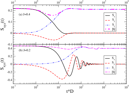
So far, we have only focused on the spin relaxation from a spin-polarized state along the -axis. Precession of the spin around an external field requires a magnetization perpendicular to this external field. To accomplish this, we applied a finite magnetic field for to induce a magnetization in -direction. At , the external field is rotated in -direction. In the absence of any relaxation mechanism, i.e. for , the spin would only precess in the -plane once is aligned along the -axis. The finite Kondo interaction, however, induces spin flips and causes spin exchange between the conduction band and the localized spin. In the thermodynamic limit and for , the expectation value of the spin vector will evolve into a spin aligned along the -axis.
The time evolution of all spin components is displayed in Fig. 10 for a magnetic field of constant strength rotated from the - to the -axis at . Since the Zeeman term of the Hamiltonian (59) does not commute with the total and only with , the TD-NRG calculations are much more time consuming. The black and red curve (online) show the and components, respectively. As expected, the spin precesses in the -plane which is clearly visible for . In addition, these two components decay with time and vanish for long times, while the component grows and reaches a value close to the thermodynamic expectation value with respect to . This indicates clearly that the TD-NRG can covers more complex relaxation phenomena. Indeed the local expectation values tent to approach their long time thermodynamic limit, which is a highly non-trivial feature of the method.
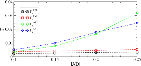
For a quantitative analysis, we fitted the two spin components and by the following phenomenological ansatz: and . shows an oscillatory behavior with a frequency for the ferromagnetic Kondo coupling and an for the anti-ferromagnetic Kondo coupling. The decay of the local component leads to a very small but finite magnetization in the conduction electron chain in direction. Its local component induces a spin precession of the which is damped by the spin-flip processes. For a chain length of , we estimate the average magnetization per chain link as which is a good estimate for the lower limit of an effective local magnetic field in direction generated by the conduction electrons in a finite size system. In the anti-ferromagnetic case, the coupling of the local spin to the conduction electrons is strongly enhanced which might cause an inhomogeneous distribution of magnetization over the Wilson chain. This effect must vanish in the thermodynamic limit . We find for and for .
In Fig. 11, the effective spin-relaxation rates and are displayed as function of for an initially decoupled local spin, i.e. . With the exception of , is smaller than for anti-ferromagnetic coupling while the transversal relaxation is always slower than the longitudinal for ferromagnetic coupling. However, the absolute values strongly depend on the fitting functions for and , so that the relaxation rates are roughly equal for all directions. Note that the usual dephasing time in NMR and ESR experiments originates from an average over signals stemming from many spins subject to local fluctuations of the externally applied field. This inhomogeneities yields the ESR condition which does not necessarily hold for the single spin decay investigated here.
VII Summary and discussion
VII.1 Discussion
We have presented a powerful novel approach to the nonequilibrium dynamics of quantum impurity systems based upon Wilson’s NRG. Its virtue is based on three key points: (i) all states of the Wilson chain are used for the time-evaluation of local operator, (ii) time expectation values can be expressed by a summation of all NRG iterations, where at each iteration the matrix elements of any local operator is weight by the reduced density matrix which contain information about dissipation and decoherence and (iii) the continuum limit of the bath is mimicked by using the -trick where the true time evolution is obtained by averaging over a different bath discretization. By its nature, it is applicable to arbitrary temperatures, and allows for the study of the temperature evolution of real-time dynamics.
We have previously established the accuracy of the approach on all time scales up to by comparison with exact solution of the RLM AndersSchiller2005 . In this paper, we additionally benchmarked our method to the exact analytical solution of the decay of the off-diagonal matrix element of the local density matrix which is taken as measure for decoherence of a spin state. This is the first application of the TD-NRG to bosonic baths. In this case, the TD-NRG is much less susceptible to discretization errors than for fermionic baths. This behavior roots in the extended number of bath states, in principle infinite, which are available for distributing energy and phase at each energy scale . From this observation, we conjecture that the TD-NRG will be even more suitable from bosonic baths than for fermionic baths. A detailed study of the real-time dynamics of the spin-boson model in the subohmic regime will be published soon. Combining fermionic and bosonic bathsGlossopIngersent2005 will open new possibilities for the description of spin decay of ultra-small quantum dots coupled to the leads as well as charge noise.
We have investigated the spin decay of the Kondo model in the ferromagnetic and in the antiferromagnetic regime. For the ferromagnetic regime, we identified a universal dimensionless time scale for the transient behavior of the spin decay. In the antiferromagnetic regime, the spin response at short time scales follows excellently the presented analytical perturbative solution which is valid up the second order in the coupling constant. At long times, the Kondo correlations dominate, and the rescaled curves appear to collapse onto a universal curve for as predicted by conformal field theory LesageSaleur1998 . At short and intermediate times , the anisotropy of and influences the time evolution and no universality is found as a one parameter scaling for different values of . This reflects the different role of and in the spin-relaxation process. The spin relaxation is governed by the spin-flip term and not by which only enters through renormalization in higher order processes into . Only at and at infinitely long times, the anisotropy Kondo model becomes isotropic in the strong coupling fixed point. Here, we expect the validity of universal scaling.
VII.2 Outlook
The time-dependent NRG approach will open new doors to our understanding of a new class of nonequilibrium problems whose real-time dynamics is governed by a strong entanglement of the environment with the quantum-impurity states. The exact analytical solution of decoherence of a pure quantum states explicitly shows that the true dynamics is not simply given by an exponential decay rate but a function . The reproduction of these non-trivial analytical results of the spin-boson model with all details reveals already the strong potential of our method. The application to charge-transfer reactions in biological systemsTornowBulla2005 influenced by the molecular vibrations is subject of an ongoing research project. We hope that this will ultimately lead to a better understanding how secondary and tertiary molecular structures of protein molecules influence the chemistry and, therefore, the functionality of such proteins. It was pointed out by Schulten Schulten2000 that the chemical structure of reaction centers in protein molecules by itself does not give us the desired understanding why thermal fluctuations do no harm the deterministic outcome of the complex cellular chemistry which is the basis of existence of living organisms.
We have benefited from discussions with G. Alber, R. Bulla, G. Czycholl, T. Costi, S. Kehrein, A. Hewson, E. Lebanon, A. Rosch, K. Schönhammer, S. Tornow, D. Vollhardt, M. Vojta and A. Weichselbaum. F.B.A. acknowledges funding of the NIC, Forschungszentrum Jülich under project no. HHB000, and DFG funding under project AN 275/5-1. A.S. was supported in part by the Centers of Excellence Program of the Israel Science Foundation.
Appendix A Calculation of the overlap matrix elements
In this appendix, we describe in detail the calculation of the overlap matrix elements of Eq. (34). We need the matrix element
| (74) |
in order to calculate the reduced density matrix in basis of the Hamiltonian needed in Eq. (35). Here, is an eigenstate of and an eigenstate of and the environment variable has been droped for simplicity. Independent of the dynamics of , the original basis of the Hamiltonian matrices and is identical prior to diagonalization. Therefore, the overlap is given by
| (75) |
where labels the states on the impurity. Let us assume, we know all matrix elements at iteration . Then, the NRG recursion relation adds the same degrees of freedom to the new chain of length , independent of the dynamics of . Since the new eigenstates can be expanded into
| (76) | |||||
| (77) |
the matrix element is given by
In combination with the initial condition (75), Eq. (A) defines a recursion relation from which all overlap matrix elements are obtained.
References
- (1) D. C. Langreth and J. W. Wilkins, Phys. Rev. B 6, 3189 (1972).
- (2) L. P. Kadanoff and G. Baym, Quantum Statistical Mechanics (Benjamin, New York, 1962).
- (3) L. V. Keldysh, Sov. Phys. JETP 20, 1018 (1965).
- (4) K. G. Wilson, Rev. Mod. Phys. 47, 773 (1975).
- (5) H. R. Krishna-murthy, J. W. Wilkins, and K. G. Wilson, Phys. Rev. B 21, 1003 (1980).
- (6) H. R. Krishna-murthy, J. W. Wilkins, and K. G. Wilson, Phys. Rev. B 21, 1044 (1980).
- (7) D. M. Cragg and P. Lloyd, J. Phys. C 12, 3301 (1979).
- (8) H. B. Pang and D. L. Cox, Phys. Rev. B 44, 9454 (1991).
- (9) B. A. Jones and C. M. Varma, Phys. Rev. Lett. 58, 843 (1987).
- (10) B. A. Jones, C. M. Varma, and J. W. Wilkins, Phys. Rev. Lett. 61, 125 (1988).
- (11) O. Sakai, Y. Shimizu, and T. Kasuya, Solid State Commun. 75, 81 (1990).
- (12) O. Sakai and Y. Shimizu, J. Phys. Soc. Jap. 61, 2333 (1992).
- (13) O. Sakai and Y. Shimizu, J. Phys. Soc. Jap. 61, 2343 (1992).
- (14) K. Ingersent, B. A. Jones, and J. W. Wilkins, Phys. Rev. Lett. 69, 2594 (1992).
- (15) F. B. Anders and A. Schiller, Phys. Rev. Lett. 95, 196801 (2005).
- (16) T. A. Costi, Phys. Rev. B 55, 3003 (1997).
- (17) R. P. Feynman, Statistical Mechanics, A Set of Lectures (Benjamin, Reading, MA, 1972).
- (18) W. Hofstetter, Phys. Rev. Lett. 85, 1508 (2000).
- (19) R. Bulla, N. Tong, and M. Vojta, Phys. Rev. Lett. 91, 170601 (2003).
- (20) F. Verstraete et al., Variational matrix product state approach to quantum impurity models, cond-mat/0504305, 2005.
- (21) M. A. Cazalilla and J. B. Marston, Phys. Rev. Lett. 88, 256403 (2002).
- (22) A. J. Daley, C. Kollath, U. Schollwöck, and G. Vidal, J. Stat. Mech.: Theor. Exp. P04005 (2004).
- (23) S. R. White and A. E. Feiguin, Phys. Rev. Lett. 93, 076401 (2004).
- (24) D. Gobert, C. Kollath, U. Schollwoeck, and G. Schuetz, cond-mat/0409692, (2004).
- (25) U. Schollwöck, Rev. Mod. Phys. 77, 259 (2005).
- (26) M. Yoshida, M. A. Whitaker, and L. N. Oliveira, Phys. Rev. B 41, 9403 (1990).
- (27) S. Tornow, N.-H. Tong, and R. Bulla, Europhys. Lett. 73, 913 (2006).
- (28) A. J. Leggett, S. Chakravarty, A. T. Dorsey, and M. P. A. Fisher, Rev. Mod. Phys. 59, 1 (1987).
- (29) U. Weiss, Quantum Dissipative Systems (World Scientific, Singapure, 1999).
- (30) D. Xu and K. Schulten, Chemical Physics 91, 170601 (1994).
- (31) K. Schulten, Science 290, 61 (2000).
- (32) R. A. Marcus, Rev. Mod. Phys. 65, 599 (1993).
- (33) W. G. Unruh, Phys. Rev. A 51, 992 (1995).
- (34) G. M. Palma, K.-A. Suominen, and A. K. Ekert, Proc. R. Soc. Lond. A 452, 567 (1996).
- (35) R. Bulla, H.-J. Lee, N.-H. Tong, and M. Vojta, Phys. Rev. B 71, 045122 (2005).
- (36) P. Nordlander, M. Pustilnik, Y. Meir, and N. S. Wingreen, Phys. Rev. Lett. 83, 808 (1999).
- (37) P. W. Anderson, J. Phys. C 3, 2436 (1970).
- (38) A. C. Hewson, The Kondo Problem to Heavy Fermions (Cambridge Press, Cambridge UK, 1993).
- (39) D. Lobaskin and S. Kehrein, Phys. Rev. B 71, 193303 (2005).
- (40) F. Wegner, Ann. Physik 3, 77 (1994).
- (41) M. T. Glossop and K. Ingersent, Phys. Rev. Lett. 95, 67202 (2005).
- (42) F. Lesage and H. Saleur, Phys. Rev. Lett. 80, 4371 (1998).