Opposite spin accumulations on the transverse edges by the confining potential

Abstract

We show that the spin-orbit interaction induced by the boundary confining potential causes opposite spin accumulations on the transverse edges in a zonal two-dimensional electron gas in the presence of external longitudinal electric field. While the bias is reversed, the spin polarized direction is also reversed. The intensity of the spin accumulation is proportional to the bias voltage. In contrast to the bulk extrinsic and intrinsic spin Hall effects, the spin accumulation by the confining potential is almost unaffected by impurity and survives even in strong disorder. The result provides a new mechanism to explain the recent experimental data.

I Introduction

Recently, two experimental groups observed the transverse opposite spin accumulations near two edges of their devices in the presence of a longitudinal voltage bias.experiment1 ; experiment2 One experiment is on n-type GaAs’s bar with a size about $300\mu m\times 77\mu m$,experiment1 and the spin accumulation is detected by Kerr rotation spectroscopy. The other experiment is on a coplanar p-n junction light-emitting diode device.experiment2 Under a longitudinal bias, a circular polarization of the emitting light on two edges is detected. The directions of the polarization are opposite on the two edges, which suggests opposite spin accumulation on the two edges. Moreover, when the bias is reversed, the spin accumulations are reversed in the above two experiments.

These experiments originally were motivated to measure the predicted effects: the extrinsic and intrinsic spin Hall effects (SHE). The extrinsic SHE has been discovered about a few decades ago,eshe1 ; eshe2 and it originates from the spin dependent scattering that deflects the spin-up and spin-down carriers towards the opposite edges of a sample. The intrinsic SHE is predicted first by Murakami et.al. and Sinova et.al. in a Luttinger spin-orbit (SO) coupled 3D p-doped semiconductorZhangsc and a Rashba SO coupled two-dimensional electron gas (2DEG)Sinova , respectively. Recently, a number of sequent works have focused on this interesting effect.SHE1 ; SHE2 ; SHE3 ; SHE4 Nonetheless, the intrinsic SHE still remains a controversy topic. The intrinsic spin Hall conductivity originally was pointed out to be universal in the clean bulk sample.Sinova However some works have showed that the spin-Hall conductivity depends on the SO coupling strength and electron Fermi energy in general.SHE1 Moreover, it has been shown recently that the impurity plays an important role on the intrinsic SHE. In an infinite system, it has been shown that the spin Hall conductivity is very sensitive to disorder.SHE2 The effect vanishes even in a very weak disorder limit when the vertex correction is considered. In a finite mesoscopic ballistic system, the SHE can survive.SHE3 The SHE and spin accumulations have been studied in the dirty or clean finite mesoscopic samples by using the Landauer-Büttiker formalism and the tight-binding HamiltonianDattabook . These works show that the opposite spin accumulations indeed can generate on the transverse two edges in the finite system, and the SHE still presents below a critical disorder threshold.SHE3

Although the spin accumulation observed in the two experiments appears to reflect the physics of the SHE, there is still a significant challenge to explain the observed experiment effect. The spin accumulation contributed from the extrinsic SHE has been shown to have the directions of spin polarization that are opposite to the experimental results.SHE2 While the intrinsic SHE is predicted to have the same directions of spin polarization as that observed in the experiments, it is expected to be scaled with length and eventually be vanished in Rashba spin orbit coupling systems in the presence of disorder. Since the experiments are not done in the ballistic region and the signal of spin accumulation has little dependence of the transversal length of the sample, it is not clear that how the intrinsic SHE explains all experimental results solely.

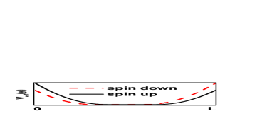
Figure 1: (Color online) Schematic diagram for the transverse effective potential $V_{eff}(y)$ in the zonal 2DEG for the positive $+p_{x}$.

In this paper, we give a new mechanism that can generate the opposite spin accumulations in two edges under the longitudinal voltage bias. We first show the principle of this new mechanism. Considering an infinite zonal 2DEG with a confining potential on $y$-direction, which is described by the Hamiltonian $H$: $H=\frac{p_{x}^{2}+p_{y}^{2}}{2m^{*}}+V(y)$, where $p_{x/y}$ is the momentum operator and $m^{*}$ is the effective mass of electrons. $V(y)$ is the confining potential energy which is constant in the center and quickly increases as tending to the boundary. Based on the relativity effect, in the presence of the internal electric field ${\bf E}=\nabla V(y)/e$, there is a natural spin-orbit coupling term $V_{SO}=\frac{e\hbar}{2m^{*2}c^{2}}\;\sigma\cdot({\bf E}\times{\bf p})$.book ; sun Considering that the corresponding electric field ${\bf E}=\nabla V(y)/e$ is perpendicular to the edge, only the element $E_{y}$ of $y$-direction is non-zero and the spin-orbit coupling energy reduces into: $V_{SO}=-\frac{\hbar}{2m^{*2}c^{2}}\;\sigma_{z}p_{x}\frac{d}{dy}V(y)$. So for the spin-down ($\sigma_{z}=\downarrow$ or $-1$) electrons, its effective potential $V_{eff}(y)=V(y)+V_{SO}(y)$ is lower than the one of spin-up electrons at the edge of $y=0$ for positive $+p_{x}$ (see Fig.1). On the other hand, at the other edge of $y=L$, the effective potential $V_{eff}$ of the spin-up electrons is lower for $+p_{x}$ (see Fig.1). Thus, the spin accumulations on the two transverse edges form when electrons occupy the positive $+p_{x}$ states under the positive longitudinal bias. When the bias is reversed, the electrons occupy the negative $-p_{x}$ state and the spin accumulation reverses its sign. Therefore it produces the same spin accumulation as that observed in the experiments.experiment1 ; experiment2 In the present model, the spin accumulation originates completely from the structure confining potential, so it is not affected by the impurity and the dephase. In a word, the structure confining potential can also induce the opposite spin accumulation, which can be the origin of the experimentally observed spin accumulation.

The paper is organized as follows: in section II, we will mention and solve the model in detail. The results and discussions are in section III. Finally, a brief summary is given in section IV.

II The model and solution

The Hamiltonian of the zonal 2DEG can be written as:

$$H=\frac{p_{x}^{2}+p_{y}^{2}}{2m^{*}}+V(y)-\frac{\hbar}{2m^{*2}c^{2}}\;\sigma_{z}p_{x}\frac{d}{dy}V(y).$$ (1)

Here the first term is kinetic energy, the second term is the potential energy, and the third term is from the spin-orbit coupling energy due to the boundary confining potential $V(y)$ as mentioned in the introduction.

Due to the fact $[p_{x},H]=0$ and $[\sigma_{z},H]=0$, $k_{x}$ and $\sigma_{z}$ are the good quantum numbers, the eigenstates in such a structure can be written in the form $\Psi(x,y)=\phi_{nk_{x}}(y)exp(ik_{x}x)$ with the dispersion relation $E=\epsilon_{nk_{x}}+\hbar^{2}k_{x}^{2}/2m^{*}$. The index $n$ numbers the different subbands with the wave-function $\phi_{nk_{x}}(y)$ in the $y$-direction and a energy $\epsilon_{nk_{x}}$, which are functions of the wave vector $k_{x}$. The transverse wave-function $\phi_{nk_{x}}(y)$ satisfies the equation:

$$\left[\frac{p_{y}^{2}}{2m^{*}}+V(y)-\gamma\sigma_{z}\frac{dV(y)}{dy}\right]\phi_{nk_{x}}(y)=\epsilon_{nk_{x}}\phi_{nk_{x}}(y),$$ (2)

where $\gamma=\frac{\hbar^{2}k_{x}}{2m^{*2}c^{2}}$. In the experiment, the length $L$ along the transverse $y$-direction is very long [e.g. in the order of tens of micron in Ref.(1)] while the confining potential is only limited in several atom’s layers. So we model this potential $V(y)$ as a square potential well, i.e. $V(y)=0$ for $0<y<L$ and $V(y)=V$ for others $y$. In this case, $V_{SO}=-\gamma\sigma_{z}\frac{d}{dy}V(y)$ becomes the $\delta$-function. The Hamiltonian can be solved analytically, and the Schrödinger equation Eq.(2) for the spin-up electron reduces into:

$$[\frac{p_{y}^{2}}{2m^{*}}+V(y)+\gamma(\;\delta(y)-\delta(y-L)\;)\;]\phi(y)=\epsilon\phi(y).$$ (3)

The spin-down electronic Schrödinger equation is same to Eq.(3) except $\gamma\rightarrow-\gamma$. The wave function $\phi(y)$ in Eq.(3) can be written as:

$$\phi(y)=\left\{\begin{array}[]{ll}Ae^{\beta y},&~{}~{}y<0\\ sin(k_{y}y+\theta),&~{}~{}0<y<L\\ Be^{-\beta y},&~{}~{}y>L\end{array}\right.$$

where $k_{y}=\sqrt{2m^{*}\epsilon}/\hbar$, $\beta=\sqrt{2m^{*}(V-\epsilon)}/\hbar$, and $A$, $B$, and $\theta$ are the constants to be determined by the boundary conditions. Here the boundary conditions are $\phi(y)|_{y=0^{-}/L^{-}}=\phi(y)|_{y=0^{+}/L^{+}}$ and $\phi^{\prime}(y)|_{y=0^{+}/L^{+}}-\phi^{\prime}(y)|_{y=0^{-}/L^{-}}=\pm(2m^{*}\gamma/\hbar^{2})\phi(y)|_{y=0/L}$, which lead to

$$\left\{\begin{array}[]{l}sin\theta=A\\ sin(k_{y}L+\theta)=Be^{-\beta L}\\ k_{y}cos\theta-A\beta=2m^{*}\gamma A\\ \beta Be^{-\beta L}+k_{y}cos(k_{y}L+\theta)=2m^{*}\gamma Be^{-\beta L}\end{array}\right.$$

Solving the equation set, we get $\epsilon_{nk_{x}}$ and $\phi_{nk_{x}}(y)$. Sequentially the spin-up electron probability distribution $P_{nk_{x},\uparrow}(y)=|\phi_{nk_{x}}(y)|^{2}$ is obtained. The same calculation can be done for the spin-down electron. Due to the system is universal along the $x$-direction, and the spin accumulation is independent of $x$, $P_{nk_{x},\uparrow\downarrow}(y)$ completely describes spin distribution.

Although the square confining potential $V(y)$ model is solvable analytically, the potential in the real system is not abrupt. An gradual change from bottom to top close to the interface is expected. For this reason, we consider the real parabolic confining potential $V(y)$ and solve the system numerically by using the tight-binding HamiltonianDattabook . In addition, we also study the disorder effect on the spin accumulations. In the tight-binding approximation, the Hamiltonian in Eq.(2), which is related to $y$-direction, can be written as the following discrete lattice version:

$$H=\sum\limits_{i,\sigma}(\epsilon_{i}+V_{i}+\sigma_{z}V_{SO,i})a_{i\sigma}^{\dagger}a_{i\sigma}+\sum\limits_{<ij>,\sigma}t\;a_{i\sigma}^{\dagger}a_{j\sigma},$$ (4)

where $\sigma=\uparrow,\downarrow$ (or $\pm 1$) is the spin index in $z$-direction, and $t=\hbar^{2}/2m^{*}a^{2}$ represents the hopping matrix element with the lattice constant $a$. The confining potential $V(y)$ is assumed to be parabolic: $V(y)=V\frac{(y-6a)^{2}}{25a^{2}}$ for $a\leq y\leq 5a$, $V(y)=0$ for $5a<y\leq L-5a$, and $V(y)=V\frac{(y-L+5a)^{2}}{25a^{2}}$ for $L-5a<y\leq L$. For a clean system, the onsite energy $\epsilon_{i}=0$, and $\epsilon_{i}$ is randomly distributed between [$-W/2,W/2$] for the dirty system. The Hamiltonian in Eq.(4) can easily be solved by numerically calculating the eigenvalues and eigenstates of the Hamiltonian matrix. Due to decoupling between the different spin states in the Hamiltonian, we can solve the eigenvalues and eigen-wavefunctions separately for the spin-up and spin-down electrons. Whereafter, the the spin-up and spin-down electron probability distribution $P_{nk_{x},\sigma}(i)$ in the subband $n$ and the longitudinal momentum $\hbar k_{x}$ is obtained straightforwardly.

While the longitudinal bias is zero, the spin accumulations $S(y)$ is zero everywhere, because of the existence of the time-reversal invariance. On the other hand, when a bias $V_{bias}$ is added, the spin accumulations $S(y)$ will emerge. Consider the device under the positive bias $V_{bias}$ and at the zero temperature, the $+k_{x}$ states with its energy between $E_{f}-V_{bias}/2$ and $E_{f}+V_{bias}/2$ are occupied by electrons, while the states for the negative $-k_{x}$ are empty, here $E_{f}$ is the Fermi energy. Then, under the small bias and taking the linear approximation, the spatial density distribution $P_{\uparrow\downarrow}(i)$ of the spin-up (down) electrons along $y$-direction for the unit bias is $P_{\uparrow\downarrow}(i)=\sum_{n}\rho_{n}(E_{k_{x}})P_{nk_{x},\uparrow}(i)$, where $\rho_{n}(E_{k_{x}})$ is the density of state in the subbands $n$ with $E_{k_{x}}=E_{f}-\epsilon_{nk_{x}}$, and the sum is over all subbands $n$ with its cut-off energy lower than $E_{f}$. The spin accumulation density and charge density in the linear bias can be obtained as: $P_{s}(i)\equiv\lim_{V_{bias}\rightarrow 0}\frac{S(ia)}{V_{bias}}=\frac{\hbar}{2}(P_{\uparrow}(i)-P_{\downarrow}(i))$ and $P_{e}(i)=e(P_{\uparrow}(i)+P_{\downarrow}(i))$.

In the numerical calculation, we choose the realistic parameters as ones in the experiment:Gui the electronic effective mass $m^{*}=0.05m_{e}$ and the Fermi energy $E_{f}=0.1eV$, in which the corresponding electron concentration is approximately $n_{2D}=10^{12}cm^{-2}$. The energy unit is set to $1eV$, and the length unit is $1nm$ for the analytic model, or $1a.u.$ for the tight-banding model. The lattice constant $a$ in the tight-banding model is around $0.196nm$.

III numerical results and discussion

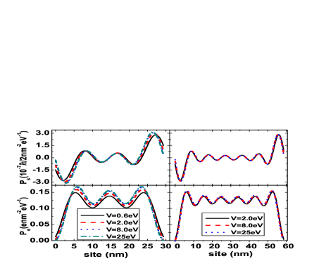
Figure 2: (Color online) The transverse distribution of the spin and charge density, $P_{s}(y)$ and $P_{e}(y)$, vs $y$ for the square confining potential. Left panel: $L=29.3nm$, right panel: $L=58.6nm$.

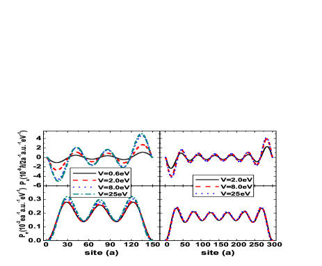
Figure 3: (Color online) The transverse distribution of the spin and charge density, $P_{s}(y)$ and $P_{e}(y)$, vs $y$ for the parabolic confining potential. Left panel: $L=150a$, right panel: $L=300a$.

First, we study spin accumulation in the clean system. In the present system, the spin accumulation density $P_{s}(y)$ depends on the transverse position $y$, and it is independent of the longitudinal position $x$. Fig.2 and Fig.3 show the spin accumulation density $P_{s}(y)$ and charge density $P_{e}(y)$ versus $y$ for the case of the square and the parabolic confining potential $V(y)$, respectively. First of all, the opposite spin accumulations at $z$-direction indeed are generated near the two edges regardless of the square or the parabolic potential. If the bias is reversed, the electrons occupy the negative $-k_{x}$ states instead of the positive $+k_{x}$ states and the spin accumulations also are reversed. These results are consistent with the experimental results.experiment1 ; experiment2 The opposite spin accumulations here obviously originates from the confining potential as mentioned in the introduction because there is no other interaction except for the potential $V(y)$. Second, the spin accumulations mainly are near the two edges, and it is small and has oscillation in the bulk. The oscillation is expected due to the existence of Fermi surface. The period is given by $2\pi/k_{F}$. For a fixed Fermi energy (e.g. $E_{f}=0.1eV$), the wider the width $L$ is, the more the subbands below $E_{f}$ will be. At the mean time, the oscillation times of $P_{s}$ and $P_{e}$ are more and the oscillation amplitude are smaller. So the bulk $P_{s}$ almost vanishes and $P_{e}$ approaches constant at large $L$. But the spin accumulations near the edge, including the intensity and the location, is almost independent with $L$. Third, we discuss the characters of the spin accumulations $P_{s}(y)$ as a function of the strength $V$ of the confining potential $V(y)$. The characters are slightly different for the square and parabolic potentials. While $V=0$, $P_{s}(y)=0$ for both the square and parabolic potentials. With $V$ increasing, $P_{s}(y)$ emerges. For the square potential, $P_{s}(y)$ quickly arises in the beginning. Around $V=5E_{f}$, $P_{s}(y)$ has reached saturated value. Thereafter the value almost does not change with further increasing $V$ (see Fig.2a,b). For the parabolic potential, $P_{s}(y)$ increases slowly. Around $V=8eV$, it saturates. For comparison, we also show the charge density $P_{e}(y)$ in Fig.2 and Fig.3. Here $P_{e}(y)>0$ in any position $y$, and $P_{e}(y)$ is symmetric while $P_{s}(y)$ is asymmetric.

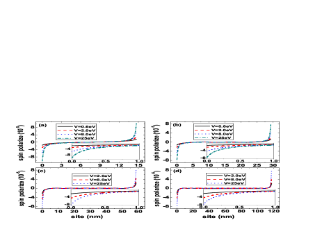
Figure 4: (Color online) The spin polarization $P_{s}/P_{e}$ ${\sl vs}$ the transverse site $y$ for the square confining potential. Panel (a),(b),(c),(d) correspond to $L=14.6nm$, $L=29.3nm$, $L=58.6nm$, and $L=117.3nm$, respectively. The insets show the detailed distribution near the edge of $y=0$ in the central panel.

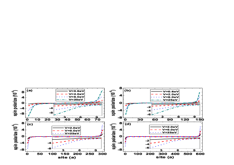
Figure 5: (Color online) The spin polarization $P_{s}/P_{e}$ ${\sl vs}$ the transverse site $y$ for the parabolic confining potential. Panel (a),(b),(c),(d) correspond to $L=75a$, $L=150a$, $L=300a$, and $L=600a$, respectively. The insets show the detailed distribution near the edge of $y=0$ in the central panel.

Next, we discuss the spin polarization $P_{s}(y)/P_{e}(y)$. In the central panel of Fig.4 and Fig.5, we plot the transverse distribution of the spin polarization for the square and parabolic confining potential $V(y)$, respectively. It is clearly shown that the opposite spin polarization emerges on the transverse two edges whatever $L$ is set. For example, in the Fig.4 and 5, the transverse width $L$ is set to $14.6nm$, $29.3nm$, $58.6nm$ and $117.3nm$ which is very different, but the spin polarization distributions near the edge are almost identical. In addition, the spin polarization on the transverse edge is close to a linear function as $V$ while $P_{s}(y)$ is hardly affected by the strength of $V$ (see Fig.2 and 3). The detailed distributions of the spin polarization near the edge of $y=0$ are magnified and shown in the insets (in Fig.4 and 5). The distribution range for the parabolic potential is slightly wider than that for the square potential because the variation range of the parabolic potential $V(y)$ is wider than that of the square potential $V(y)$.

The above result is obtained in a clean system. In the following, we study the spin accumulation in the dirty system. Fig.6 displays the transverse distribution of $P_{s}(y)$, $P_{e}(y)$ and spin polarization $P_{s}(y)/P_{e}(y)$ with different disorder strength $W=0.1E_{f},1E_{f},2E_{f}.5E_{f},10E_{f}$. In these calculation, $P_{s}(y)$ and $P_{e}(y)$ are obtained by averaging over up to 5000 realizations of disorder. From Fig.6, we can see that the spin accumulation $P_{s}(y)$ and the spin polarization near the two edges are almost unaffected by the disorder, even the disorder $W$ is very strong (e.g. $W=10E_{f}$). In fact, the spin accumulation in the present device originates from the confining potential near the edge, where the effective potentials for spin-up and spin-down electrons are different (see Fig.1). Intuitively, the spin polarization is expected to be unaffected by the disorder as well as the dephase. Additionally, with the increasing of the disorder $W$, the amplitudes of the oscillation of $P_{e}(y)$ and $P_{s}(y)$ in the bulk are slightly reduced (see Fig.6a,b), and their fluctuations are increased linearly.

To compare our numerical results with the experiment experiment1 , we calculate the value for spin polarization and accumulation. From the experimental data, the spin density at the peak can be estimated: $P_{s}\approx(1.5--4.2)\times 10^{-6}nm^{-2}eV^{-1}$, and the spin polarization is $(1.0--2.8)\times 10^{-4}$ for a thickness $h=0.9\mu m$. From figures (e.g. fig.2 and fig.4), our calculation show that the peak spin density $P_{s}\approx 0.3\times 10^{-6}nm^{-2}eV^{-1}$ and the spin polarization is $0.8\times 10^{-4}$. The value of the spin polarization is comparable with the experiment. Due to the big thickness in the expriment, the spin accumulation $P_{s}$ in our calculation seems to be several times smaller than that of the experiment. Indeed, a more precise quantitative calculation perhaps requires to consider the spin orbit coupling in the bulk and spin relaxation effect at the boundary. However, our simple model indeed produces the same order of magnitude as one measured in the experiments.

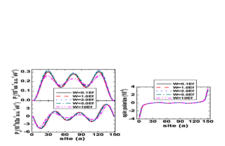
Figure 6: (Color online) The charge density distribution $P_{e}$ (a), the spin density distribution $P_{s}$ (b), and spin polarization $P_{s}/P_{e}$ (c) ${\sl vs}$ the transverse site $y$ for the different disorder $W$, respectively. The other parameters are: $E_{f}$=0.1eV, $L=150a$, and $V=8eV$.

IV Conclusion

In summary, we propose a new mechanism to explain the spin accumulations at the edges of a zonal two dimensional electron system. Due to the strong structure confining potential in the boundary, the induced spin-orbit interaction leads to the opposite spin accumulation on the two transverse edges under the longitudinal voltage bias. The spin polarized direction can be reversed while the bias is reversed. The intensity of the polarization is also proportional to the external longitudinal voltage bias. These results are consistent with the recent experiment. Moreover, the experimental test of the new mechanism can be easily performed in future experiments. Unlike the extrinsic and intrinsic SHE, the spin accumulations in the present mechanism are hardly affected by the disorder and dephase, and can exist even in the strong disorder system.

References

- (1) Electronic address: sunqf@aphy.iphy.ac.cn
- (2) Electronic address: hu4@physics.purdue.edu
- (3) Y.K. Kato, R.C. Myers, A.C. Gossard, and D.D. Awschalom, Science 306, 1910 (2004); V. Sih, R.C. Myers, Y.K. Kato, W.H. Lau, A.C. Gossard, and D.D. Awschalom, Nature Phys. 1, 31 (2005).
- (4) J. Wunderlich, B. Kaestner, J. Sinova, and T. Jugwirth, Phys. Rev. Lett., 94, 047204 (2005).
- (5) M.I. Dyakonov and V.I. Perel, JETP Lett. 13, 467 (1971); Phys. Lett. A 35, 459 (1971).
- (6) J.E. Hirsch, Phys. Rev. Lett. 83, 1834 (1999).
- (7) S. Murakami, N. Nagaosa, and S.C. Zhang, Science 301, 1348 (2003); Phys. Rev. B 69, 235206 (2004).
- (8) J. Sinova, D. Culcer, Q. Niu, N.A. Sinitsyn, T. Jungwirth, and A.H. MacDonald, Phys. Rev. Lett. 92, 126603 (2004).
- (9) E.M. Hankiewicz, L.W. Molenkamp, T. Jungwirth, and J. Sinova, Phys. Rev. B, 70, 241301 (2004); B.K. Nikoli, L.P. Zrbo, and S. Souma, Phys. Rev. B 72, 075361 (2005); A. Reynoso, Gonzalo Usaj, and C.A. Balseiro, cond-mat/0511750.
- (10) J.I. Inoue, G.E.W. Bauer, and L.W. Monlenkamp, Phys. Rev. B 70, 041303(R) (2004); E.G. Mishchenko, A.V. Shytov, and B.I. Halperin, Phys. Rev. Lett. 93, 226602 (2004).
- (11) J.-P. Hu, B. A. Bernevig, and C.-J. Wu, Int. J. Mod. Phys. B. 17, 5991(2003); L. Sheng, D. N. Sheng, and C.S. Ting, Phys. Rev. Lett. 94, 016602 (2005); L. Sheng, D. N. Sheng, C.S. Ting, and F.D.M. Haldane, ibid., 95, 136602 (2005); C.P. Moca, and D.C. Marinescu, Phys. Rev. B 72, 165335 (2005); J. Li, L. Hu, and S.-Q. Shen, Phys. Rev. B 71, 241305(R), (2005); B.K. Nikoli, S. Souma, L.P. Zrbo, and J. Sinova, Phys. Rev. Lett. 95, 046601 (2005); J. Yao and Z.Q. Yang, Phys. Rev. B 73, 033314 (2006); J. Wang, K.S. Chan, and D.Y. Xing, Phys. Rev. B 73, 033316 (2006).
- (12) Y. Yao and Z. Fang, Phys. Rev. Lett. 95, 156601 (2005); Z.F. Jiang, R.D. Li, S.-C. Zhang, and W.M. Liu, Phys. Rev. B 72, 045201 (2005); O. Chalaev, and D. Loss, Phys. Rev. B 71, 245318 (2005); B.A. Bernevig, and S.C. Zhang, Phys. Rev. Lett. 95, 016801 (2005); R. Raimondi and P. Schwab, Phys. Rev. B 71, 033311 (2005).
- (13) Chapter 2 and 3, in Electronic Transport in Mesoscopic Systems, edited by S. Datta (Cambridge University Press 1995).
- (14) J.D. Bjorken and S.D. Drell, Relativistic Quantum Mechanics, (McGraw-Hill, New York, 1965).
- (15) Q.F. Sun, J. Wang, and H. Guo, Phys. Rev. B, 71, 165310 (2005).
- (16) Y.S. Gui, C.R. Becker, N. Dai, J. Liu, Z.J. Qiu, E.G. Novik, H. Schäfer, X.Z. Shu, J.H. Chu, H. Buhmann, and L.W. Molenkamp, Phys. Rev. B 70,115328 (2004).