Muon spin rotation measurements of the vortex state in vanadium: A comparative analysis using iterative and analytical solutions of the Ginzburg-Landau equations

Abstract

We report muon spin rotation measurements on a single crystal of the marginal type-II superconductor V. The measured internal magnetic field distributions are modeled assuming solutions of the Ginzburg-Landau (GL) equations for an ideal vortex lattice obtained using (i) an iterative procedure developed by E.H. Brandt, Phys. Rev. Lett. 78, 2208 (1997) and (ii) a variational method. Both models yield qualitatively similar results. The magnetic penetration depth $\lambda$ and the GL coherence length $\xi$ determined from the data analysis exhibit strong field dependences, which are attributed to changes in the electronic structure of the vortex lattice. The zero-field extrapolated values of $\lambda$ and the GL parameter $\kappa$ agree well with values obtained by other experimental techniques that probe the Meissner state.

I Introduction

In order to analyze muon spin rotation ($\mu$SR) measurements on a type-II superconductor in the vortex state, it is necessary to assume a theoretical model for the spatial variation of the local internal magnetic field $B({\bf r})$.SonierRMP An essential requirement of the model is that it must account for the finite size of the vortex cores. Thus far the internal magnetic field distribution $n(B)$ measured by $\mu$SR has been analyzed assuming analytical models for $B({\bf r})$ based on London and Ginzburg-Landau (GL) theories. Since London theory does not account for the finite size of the vortex cores, a cutoff factor derived from GL theory must be inserted into the analytical London expression for $B({\bf r})$ to correct for the divergence of $B({\bf r})$ as $r\!\rightarrow\!0$. Unfortunately, analytical cutoff factors are derivable from GL theory only near the lower and upper critical fields, $B_{c1}$ and $B_{c2}$. At intermediate fields, these analytical cutoffs deviate substantially from the precise numerical calculations,Oliveira:98 making modified London models inappropriate for the analysis of $\mu$SR data. There are several approximate analytical expressions for $B({\bf r})$ that have been derived from the GL equations.Clem:75 ; Yaouanc:97 ; Hao:91 ; Pogosov:01 For example, a variational solution of the GL equations Clem:75 ; Yaouanc:97 has proven to be a reliable model for analyzing $\mu$SR measurements on V₃Si (Ref.Sonier:04 ), NbSe₂ (Ref.Callaghan:05 ) and YBa₂Cu₃O_7-δ (Ref.Sonier:97 ; Sonier:99 ). However, this analytical GL model is strictly valid only at low reduced fields $b\!=\!B/B_{c2}$ and large values of the GL parameter $\kappa$. Thus, often used analytical models for $B({\bf r})$ have limited validity and can deviate substantially from the numerical solutions of the GL equations.

Brandt has developed an iterative method for solving the GL equations that accurately determines $B({\bf r})$ for arbitrary $b$, $\kappa$, and vortex-lattice symmetry.Brandt:97 Thus far this iteration method has not been applied to the analysis of $\mu$SR measurements of $n(B)$ in the vortex state. As a first test of this method we have chosen to study the marginal type-II superconductor vanadium (V). This rigorous analysis method is expected to be required for V, whose low value of $\kappa$ falls outside the range of validity of the analytical models. In addition, the low value of $B_{c2}$ ($\approx 0.45$ T) gives us experimental access to reduced fields which are beyond the range of validity of the analytical model.

The paper is organized as follows: Theoretical models for $B({\bf r})$ are described in Sec. II. The experimental procedures are described in Sec. III. Measurements in zero external magnetic field are presented in Sec. IV. Measurements in the vortex state are described in Sec. V and concluding remarks are given in Sec. VI.

II Theoretical models

II.1 Iterative GL solution

Here we briefly outline the iteration method presented in Ref. Brandt:97 , and correct some typographical errors contained therein. The GL equations are written in terms of the real order parameter $\omega$, the local magnetic field $B$, and the supervelocity ${\bf Q}$, which are expressed as the Fourier series

$$\omega(\mbox{\boldmath$\mathrm{r}$})=\sum_{\bf K}a_{\bf K}(1-\cos\mbox{\boldmath$\mathrm{K}$}\cdot\mbox{\boldmath$\mathrm{r}$}),$$ (1)

$$B(\mbox{\boldmath$\mathrm{r}$})=\bar{B}+\sum_{\bf K}b_{\bf K}\cos\mbox{\boldmath$\mathrm{K}$}\cdot\mbox{\boldmath$\mathrm{r}$},$$ (2)

$$\mbox{\boldmath$\mathrm{Q}$}(\mbox{\boldmath$\mathrm{r}$})=\mbox{\boldmath$\mathrm{Q}$}_{A}(\mbox{\boldmath$\mathrm{r}$})+\sum_{\bf K}b_{\bf K}\frac{\hat{\mbox{\boldmath$\mathrm{z}$}}\times\mbox{\boldmath$\mathrm{K}$}}{K^{2}}\sin\mbox{\boldmath$\mathrm{K}$}\cdot\mbox{\boldmath$\mathrm{r}$},$$ (3)

where $a_{\bf K}$ and $b_{\bf K}$ are Fourier coefficients, $\omega({\bf r})=|\psi({\bf r})|^{2}$, $\bar{B}$ is the average internal field, and $\psi({\bf r})$ is the complex GL order parameter. The “tail” of the position vector ${\bf r}\!=\!(x,y)$ is at the vortex center $(0,0)$. The local magnetic field $B$ is given in units of $\sqrt{2}B_{c}$ (where $B_{c}$ is the thermodynamic critical field) and all length scales are in units of the magnetic penetration depth $\lambda$. $\mbox{\boldmath$\mathrm{Q}$}_{A}(\mbox{\boldmath$\mathrm{r}$})$ is the supervelocity obtained from Abrikosov’s solution of the GL equations near $B_{c2}$

$$\mbox{\boldmath$\mathrm{Q}$}_{A}({\mbox{\boldmath$\mathrm{r}$}})=\frac{{\bf{\nabla}}\omega_{A}\times\hat{\mbox{\boldmath$\mathrm{z}$}}}{2\kappa\omega_{A}},$$ (4)

where $\omega_{A}({\bf r})$ is calculated from Eq. (1) using

$$a_{\bf K}^{A}=-(-1)^{\nu}\exp(-\pi\nu\sqrt{3}).$$ (5)

Here $\nu=m^{2}+mn+n^{2}$, assuming a hexagonal vortex lattice with vortex positions given by

$$\mbox{\boldmath$\mathrm{R}$}_{\mathrm{mn}}=(mx_{1}+nx_{2},ny_{2}),$$ (6)

where $m$ and $n$ are integers, $x_{1}$ is the intervortex spacing, $x_{2}=x_{1}/2$ and $y_{2}=x_{1}\sqrt{3}/2$. The spatial field profile $B({\bf r})$ was calculated at approximately 950 locations within one-quarter of the rectangular unit cell shown in Fig. 1(a).

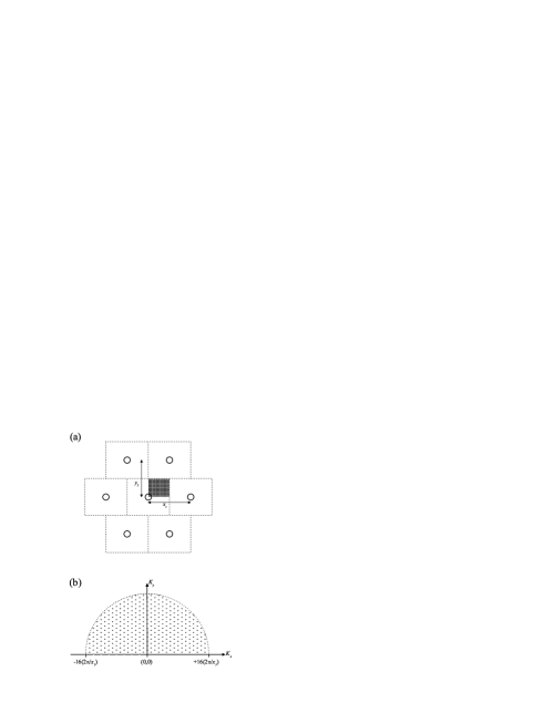
Figure 1: (a) The vortex positions in the hexagonal lattice ($\bigcirc$) and the rectangular unit cell (dotted lines). Due to symmetry, the theoretical probability field distribution $n(B)$ was calculated at approximately 950 locations ($\bullet$) within just one-quarter of the rectangular unit cell. For the sake of clarity, the sampled positions are shown at 1/4 of the density used in the calculations. (b) The points in the reciprocal space lattice ($\circ$) that are included in the ${\bf K}$ sums of Eqs. (1)–(3), Eq. (11) and Eq. (12).

The reciprocal lattice vectors used in the calcluation of $B({\bf r})$ are given by

$$\mbox{\boldmath$\mathrm{K}$}\equiv\mbox{\boldmath$\mathrm{K}$}_{\mathrm{mn}}=\frac{2\pi}{S}(my_{2},nx_{1}+mx_{2}),$$ (7)

where $S$ is the unit cell area. The $\mbox{\boldmath$\mathrm{K}$}_{\mathrm{mn}}$ vectors are restricted to those indicated in Fig. 1(b), corresponding to $-16\!\geq\!m\!\leq\!16$ and $-16\!\geq\!n\!\leq\!16$ within a semicircle with $K_{y}\geq 0$ (but excluding vectors with $K_{x}\!\geq\!0$ and $K_{y}\!=\!0$). It was found that the calculated field distribution did not change significantly if the summation was extended to values of $|n|$ and $|m|$ greater than 16.

The Fourier coefficients $a_{\bf K}$ and $b_{\bf K}$ are calculated from

$$a_{\bf K}=\frac{4\kappa^{2}<(\omega^{2}-2\omega+\omega Q^{2}+g)\cos\mbox{\boldmath$\mathrm{K}$}\cdot\mbox{\boldmath$\mathrm{r}$}>}{K^{2}+2\kappa^{2}},$$ (8)

$$a_{\bf K}=a_{\bf K}\cdot<\omega-\omega Q^{2}-g>/<\omega^{2}>,$$ (9)

$$b_{\bf K}=\frac{-2<[\omega B+\bar{\omega}(\bar{B}-B)+p]\cos\mbox{\boldmath$\mathrm{K}$}\cdot\mbox{\boldmath$\mathrm{r}$}>}{K^{2}+\bar{\omega}},$$ (10)

where $g\!=\!(\nabla\omega)^{2}/(4\kappa^{2}\omega)$, $\bar{\omega}$ is the spatial average of $\omega$ and $p\!=\!(\nabla\omega\times\mbox{\boldmath$\mathrm{Q}$})\hat{\mbox{\boldmath$\mathrm{z}$}}\!=\!Q_{y}\frac{\partial\omega}{\partial x}-Q_{x}\frac{\partial\omega}{\partial y}.$ We note that the definitions of $p$ and the $\bar{\omega}(\bar{B}-B)$ term in Eq. (10) are incorrectly written in the original article,Brandt:05 but have been corrected here. As explained in Ref. Brandt:97 , solutions to the GL equations are acquired by first iterating Eqs. (1), (8) and (9) a few times to relax $\omega$ and then iterating Eqs. (10), (1), (2), (3), (8), (9) and again (10) etc… to relax $B$.

II.2 Comparison with other models

Here we compare the results of the above iteration method for $B({\bf r})$ to the widely used modified London and analytical GL models. The local magnetic field at position ${\bf r}\!=\!(x,y)$ in the modified London modelBrandt:88 is

$$B(\mbox{\boldmath$\mathrm{r}$})=\bar{B}\sum_{\bf K}\frac{e^{-i\mbox{\boldmath$\mathrm{K}$}\cdot\mbox{\boldmath$\mathrm{r}$}}e^{-K^{2}\xi^{2}/2}}{1+\lambda^{2}K^{2}}.$$ (11)

Although this model is considered applicable for reduced fields $b\!=\!B/B_{c2}\!\leq\!0.25$ and $\kappa\!\geq\!2$, the Gaussian cutoff factor $\exp(-K^{2}\xi^{2}/2)$ introduced to account for the logarithmic divergence of $B({\bf r})$ at the center of the vortex is not strictly valid.Oliveira:98

The approximate analytical solution of the GL equations for $B({\bf r})$ isYaouanc:97

$$B(\mbox{\boldmath$\mathrm{r}$})=\bar{B}(1-b^{4})\sum_{\bf K}\frac{e^{-i\mbox{\boldmath$\mathrm{K}$}\cdot\mbox{\boldmath$\mathrm{r}$}}uK_{1}(u)}{\lambda^{2}K^{2}},$$ (12)

where

$$u^{2}=2\xi^{2}K^{2}(1+b^{4})[1-2b(1-b)^{2}].$$ (13)

$K_{1}$ is a modified Bessel function and $\xi$ is the GL coherence length. This analytical GL model is a reasonable approximation for $b\!\ll\!1$ and $\kappa\!\gg\!1$.

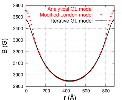
Figure 2: (Color online) The spatial field profile $B(r)$ along the straight line connecting nearest-neighbor vortices, for an hexagonal vortex lattice, $\kappa\!=\!25$, $\bar{B}\!=\!3$ kG and $\lambda\!=\!$1000 Å.

Figures 2, 3 and 4 show comparisons between the solutions for $B({\bf r})$ from the three different models, plotted along the straight line connecting nearest-neighbor vortices. The parameters used to generate the curves in Fig. 2 are characteristic of the high-$\kappa$ superconductor V₃Si (Ref.Sonier:04 ). While there is good agreement between the iterative and analytical solutions of the GL equations, the modified London model deviates substantially in the region of the vortex cores. Figure 3 shows that the modified London and analytical GL models completely break down for $\kappa\!=\!1/\sqrt{2}$, the limit of type-II superconductivity. For example, in the case of the analytical GL model, there is actually a region between the vortices where the local field changes direction. In Fig. 4, plots of $B({\bf r})$ are shown for a set of parameters obtained from $\mu$SR measurements on the low-$\kappa$ superconductor V (see Sec. V). The value $\kappa\!=\!5.3$ is rather large for V, but as we explain in Sec. V, $\kappa$ is really an “effective” fit parameter influenced by the electronic structure of the vortex lattice.

In Fig. 4 the analytical GL solution deviates from the iterative GL solution both near and far from the vortex core regions, whereas the modified London model fails only in the region of the vortex cores.

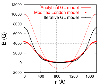
Figure 3: (Color online) The spatial field profile $B(r)$ along the straight line connecting nearest-neighbor vortices, for an hexagonal vortex lattice, $\kappa\!=\!1/\sqrt{2}$, $\bar{B}\!=\!753$ G and $\lambda\!=\!$150 Å.

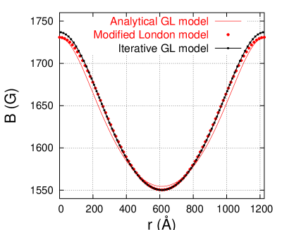
Figure 4: (Color online) The spatial field profile $B(r)$ along the straight line connecting nearest-neighbor vortices, for an hexagonal vortex lattice, $\kappa\!=\!5.3$, $\bar{B}\!=\!1.6$ kG and $\lambda\!=\!$1042 Å.

III Experimental details

The single crystal of the low-$\kappa$ superconductor V measured in the present study was purchased from Goodfellow Cambridge Ltd.Goodfellow The crystal is a disk, 13 mm in diameter by 0.35 mm thick, with the $\left<111\right>$ crystallographic direction perpendicular to the plane of the disk. Magnetization measurements indicate that the crystal has a superconducting transition temperature of $T_{c}\!=\!5.2$ K, and an upper critical field of $H_{c2}\approx 4.2$ kOe. This value of $H_{c2}$ corresponds to a BCS coherence length of $\xi_{0}\approx 280$ Å. A four-probe potentiometric ac resistivity measurement yielded $\rho=0.7$ $\mu\Omega\cdot$cm just above $T_{c}$, which is 31 times smaller than $\rho$ at rrom temperature. Using the carrier concentration $n\approx 9\times 10^{28}$ m^-3 obtained from Hall resistance measurements,Hurd a free electron theoryKittel calculation of the mean free path yields $l=\hbar k_{F}/\rho ne^{2}\approx 900$ Å, where $k_{F}=(3\pi^{2}n)^{1/3}$ is the Fermi wavenumber and $e$ is the electronic charge. Thus our sample is in the clean limit with $l/\xi_{0}\approx 3$. Neutron scattering measurements performed on our V single crystal showed no evidence of an intermediate mixed state (i.e. a mixture of Meissner and vortex-lattice phases).Forgan:05

The $\mu$SR measurements were carried out on the M15 beamline at the Tri-University Meson Facility (TRIUMF), Vancouver, Canada, using a dilution refrigerator to cool the sample. Measurements of the vortex state were done under field-cooled conditions in a “transverse field” (TF) geometry, in which the magnetic field was applied along the $z$-axis parallel to the $\left<111\right>$ direction of the crystal, but perpendicular to the initial muon spin polarization $P_{x}(0)$ (which defines the $x$-axis). Each measurement was done by implanting approximately $2\!\times\!10^{7}$ spin-polarized muons one at a time into the crystal, where their spins precess around the local magnetic field $B({\bf r})$ at the Larmor frequency $\omega=\gamma_{\mu}B$, where $\gamma_{\mu}\!=\!0.0852$ $\mu$s^-1 G^-1 is the muon gyromagnetic ratio. The muons stop randomly on the length scale of the vortex lattice, and hence evenly sample $B({\bf r})$. The $\mu$SR signal obtained by the detection of the decay positrons from an ensemble of muons implanted into the single crystal is given by

$$A(t)=a_{0}P_{x}(t)\,,$$ (14)

where $A(t)$ is called the $\mu$SR “asymmetry” spectrum, $a_{0}$ is the asymmetry maximum, and $P_{x}(t)$ is the time evolution of the muon spin polarization

$$P_{x}(t)=\int_{0}^{\infty}n(B)\cos(\gamma_{\mu}Bt+\phi)dB\,.$$ (15)

Here $\phi$ is a phase constant, and

$$n(B^{\prime})=\langle\delta[B^{\prime}-B({\bf r})]\rangle\,,$$ (16)

is the probability of finding a local field $B$ in the $z$-direction at an arbitrary position r in the $x$-$y$ plane. Further details on this application of the $\mu$SR technique are found in Ref. SonierRMP .

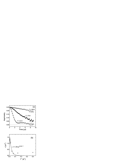
Figure 5: (a) Representative asymmetry spectra (symbols) acquired in V in zero external magnetic field, and fits (solid lines) to the numerical dynamic Gaussian Kubo-Toyabe function. (b) The temperature dependence of the extracted muon hop rate $\nu$ (circles). The solid line is a fit to $\nu(T\geq 15$ K) using an Arrhenius function.

IV Zero-field measurements

Figure 5(a) shows asymmetry spectra for our V sample in zero external magnetic field. These spectra contain a 7 % time-independent background contribution from muons stopping outside the sample. The signal coming from muons stopping inside the sample is well described by a numerical dynamic Gaussian Kubo-Toyabe function.Schenck:85 This function is characterized by a relaxation rate $\Delta$ corresponding to the width of the internal magnetic field distribution experienced by the muons, and a parameter $\nu$ corresponding to the hop rate of the muons in the sample. As shown in Fig. 5(b), the muon hop rate in our V crystal decreases with decreasing temperature to $\nu\!\approx\!0.2$ $\mu s^{-1}$ at $T=15$ K ($1/T\approx 0.07$ K^-1). At $T\geq 15$ K, the data are well described by the classical Arrhenius law for thermally activated motion in the presence of potential barriersSchenck:85

$$\nu=\nu_{0}\exp(-E_{a}/k_{B}T),$$ (17)

where $k_{B}$ is Boltzmann’s constant, $E_{a}$ is the activation energy for thermally assisted muon hopping, and $\nu_{0}$ is a constant. Fitting the $T\geq 15$ K data using this expression yields $\nu_{0}=1.72$ $\mu$s^-1 and $E_{a}=4.5$ meV. Below $T=15$ K there is perhaps a slow increase in the hop rate $\nu$, which we speculate is due to quantum mechanical tunneling as observed in other metals.Storchak

Assuming that the muon occupies an interstitial site of tetrahedral symmetry in the V crystal lattice, we can calculate the muon diffusivity $D_{\mu}$ from the expressionSchenck:85

$$D_{\mu}=\nu\frac{a^{2}}{24},$$ (18)

where $a=3.02$ Å is the lattice constant. This gives $D_{\mu}\approx 9.7\times 10^{-16}$ m²/s at $T=2.5$ K. Brandt and Seeger performed a thorough theoretical study of the effect of muon diffusion on $\mu$SR lineshapes in the vortex state.Brandt:86 They found that muon diffusion causes significant smearing of the sharp features of $n(B)$ for values of $D_{\mu}$ greater than $\approx 10^{-3}\gamma_{\mu}|M|d^{2}$, where $M$ is the sample magnetization and $d$ is the intervortex spacing. Our measured muon diffusivity is several orders of magnitude smaller than this. At $H=1.6$ kOe, for example, we have $\gamma_{\mu}|M|d^{2}\approx 2\times 10^{-8}$ m²/s, which means that $D_{\mu}(\approx 9.7\times 10^{-16}$ m²/s) $=5\times 10^{-8}\gamma_{\mu}|M|d^{2}$. Thus muon diffusion has a negligible effect on the $\mu$SR linehapes measured here.

V Measurements in the vortex state

V.1 Comparison of fits

To fit the $\mu$SR signals in the vortex state, the field distribution $n(B)$ contained in the theoretical polarization function $P_{x}(t)$ of Eq. (15) was generated from one of the three theoretical models for $B({\bf r})$ described in Sec. II. For all cases, an ideal hexagonal vortex lattice was assumed. In addition, $P_{x}(t)$ was multiplied by a Gaussian function $\exp(-\sigma^{2}t^{2}/2)$, which is equivalent to convoluting $n(B)$ with the Gaussian $\exp[-(\gamma_{\mu}B/\sigma)^{2}/2]$. This accounts for disorder in the vortex lattice,Brandt:88b and the static local-field inhomogeneity created by the large ⁵¹V nuclear dipole moments. An additional Gaussian depolarization function was added to Eq. (14) to account for approximately 20 % of the signal arising from muons that stopped outside the sample.

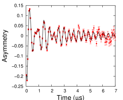
Figure 6: (Color online) Time evolution of the muon spin polarization (cirlces) in V at $H\!=\!1.6$ kOe and $T\!=\!2.6$ K, and a fit (solid curve) assuming the solution of $B({\bf r})$ from the iterative GL method.

A typical asymmetry spectrum at $H\!=\!1.6$ kOe and $T\!=\!2.6$ K is displayed in Fig. 6. The solid curve through the data is a fit assuming the solution of $B({\bf r})$ obtained from the iterative GL method. The parameter values obtained from this fit were used to calculate the spatial field profiles shown in Fig. 4. Fourier transforms of typical time domain signals and fits to both the iterative and analytical models are shown in Figs. 7 and 8. From the Fourier transforms one can see that both fits capture the main features of the $\mu$SR lineshape and are of high quality. In particular, for the data in Fig. 7 the ratio of $\chi^{2}$ to the number of degrees of freedom (NDF) is comparable, being 1.26 for the fit to the iterative GL solution and 1.30 for the fit to the analytical GL model. The values of $\lambda$, $\xi$ and $\sigma$ extracted from the two models differed by 9 %, 8 % and 13 %, respectively. We note that despite returning significantly different parameter values in some cases, fits with both models resulted in similar values of $\chi^{2}/$NDF for all of the data presented in this article.

Interestingly, the results from the two models are in slightly better agreement at the lowest temperatures and magnetic fields. For example, at $H\!=\!1.2$ kOe and $T\!=\!0.02$ K, the differences in $\lambda$, $\xi$ and $\sigma$ are 7 %, 8 % and 2 %, respectively. On the other hand, at $H\!=\!2.9$ kOe and $T\!=\!0.02$ K, $\lambda$, $\xi$ and $\sigma$ differ by 10 %, 9 % and 3 %, respectively. Even so, the quality of the fits is about the same for both models. This is evident from the Fourier transforms shown in Fig. 8. At high reduced field $b$, the values of $\lambda$ and $\xi$ obtained from the iterative GL method are likely to be more accurate, since at these high fields the analytical GL model is being applied outside its range of validity.

In the next section, complete results for fits using both the iterative and analytical GL models are presented. There we show that despite differences in the absolute values of $\lambda$ and $\xi$, fits to both models yield similar temperature and magnetic field dependences for these length scales. In particular, we show that the value of $\lambda$ extrapolated to zero field is, within experimental uncertainty, identical for both models, and furthermore agrees well with Meissner state measurements on V using other experimental techniques.

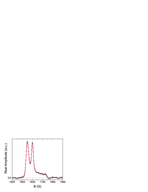
Figure 7: (Color online) Fourier transforms of the muon spin precession signal in V at $H\!=\!1.6$ kOe and $T\!=\!2.6$ K (circles), the fit using the iterative GL solution (blue curve) and the fit to the analytical GL model (red curve). The peak at 1600 G is the background signal originating from muons that missed the sample.

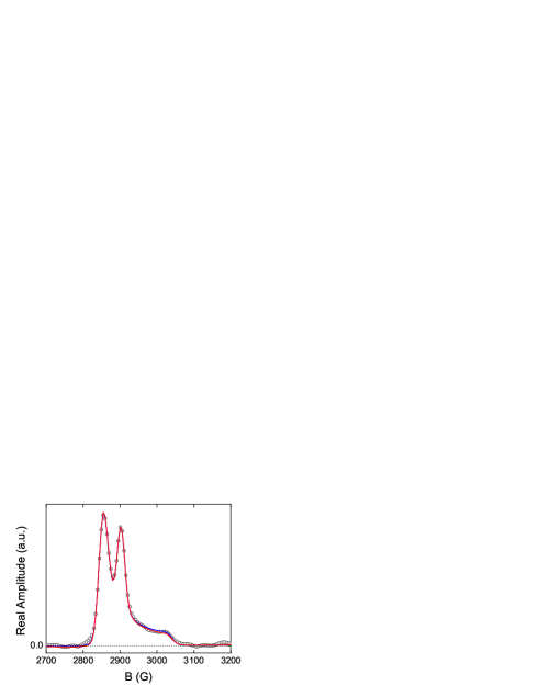
Figure 8: (Color online) Fourier transforms of the muon spin precession signal in V at $H\!=\!2.9$ kOe and $T\!=\!0.02$ K (circles), the fit using the iterative GL solution (blue curve) and the fit to the analytical GL model (red curve). The peak near 2900 G is the background signal originating from muons that missed the sample.

V.2 Temperature dependences of $\lambda$ and $\xi$

Fourier transforms of the muon spin precession signal from V at $H=1.6$ kOe and temperatures below $T_{c}$ are shown in Fig. 9. Magnetization measurements indicate that $T_{c}\!=\!3.65$ K at $H=1.6$ kOe. As the temperature is lowered, the $\mu$SR line shape broadens and the amplitude of the high-field “tail” decreases. While the high-field cutoff is less obvious at $T\!=\!0.02$ K, we note that the “true” cutoff in $n(B)$ is smeared out by the Fourier transform.SonierRMP In fact the fits in the time domain are quite sensitive to the high-field tail, yielding finite values for $\xi$, even at $T\!=\!0.02$ K.

Figure 9: Fourier transforms of the muon spin precession signal in V at $H\!=\!1.6$ kOe and $T\!<\!T_{c}(H)\!=\!3.65$ K.

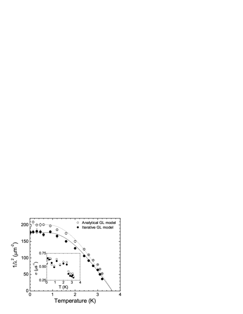
Figure 10: Temperature dependence of $1/\lambda^{2}$ in V at $H\!=\!1.6$ kOe, determined from fits using the iterative and analytical GL models. The solid and dotted curves are theoretical BCS weak-coupling predictions for $T_{c}\!=\!3.65$ K.

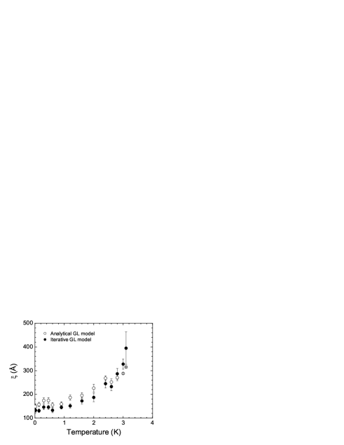
Figure 11: Temperature dependence of $\xi$ in V at $H\!=\!1.6$ kOe, determined from fits using the iterative and anlytical GL models.

Figures 10 and 11 show the temperature dependences of $1/\lambda^{2}$, $\sigma$ and $\xi$ determined from our fits of the muon spin precession signals at $H\!=\!1.6$ kOe, assuming solutions for $B({\bf r})$ from both the iterative and analytical GL methods. Despite the differences in absolute values of $1/\lambda^{2}$, both data sets in Fig. 10 are well described by BCS weak-coupling $1/\lambda^{2}(T)$ curvesMuhlschlegel:59 for $T_{c}\!=\!3.65$ K. The inset in Fig. 10 shows that both models yield similar values for the additional broadening parameter $\sigma$. As $\lambda$ becomes longer with increasing temperature, there is a greater overlap of the vortices and a corresponding reduction in the pinning-induced disorder of the vortex lattice. This is because the energy associated with the interaction between vortex lines depends on $\lambda$.Tinkham For this reason $\sigma(T)$ roughly follows $1/\lambda^{2}$ in Fig. 10.

The temperature dependence of the GL coherence length $\xi$ is shown in Fig. 11. $\xi$ is a measure of the vortex core size. Recently, we have demonstrated from $\mu$SR and thermal conductivity measurements on BCS superconductorsSonier:04 ; Callaghan:05 that the core size is dependent on the degree of localization of the quasiparticle bound core states. Thermal depopulation of the more spatially extended high-energy core states results in a shrinking of the core size with decreasing temperature. This is the so-called “Kramer-Pesch effect”,Kramer:74 which has previously been observed in NbSe₂ by $\mu$SRSonier:97 ; Miller:00 and shown to be dependent on magnetic field.Sonier:04b In a clean BCS type-II superconductor the core size of an isolated vortex is expected to be temperature independent below $T\!\sim T_{c}/k_{F}\xi_{0}$, where $k_{F}$ is the Fermi wave number and $\xi_{0}$ is the BCS coherence length. We see in Fig. 11 that $\xi(T)$ obtained from the fits to both models displays the Kramer-Pesch effect, with $\xi$ saturating below $T\approx 1$ K. Using the free-electron expression $k_{F}=(3\pi^{2}n)^{1/3}$ (Ref.Kittel ) and $n\approx 9\times 10^{28}$ m^-3 from Hall resistance measurements, Hurd we obtain $k_{F}\approx 1.4\times 10^{10}$ m^-1. Assuming the value of the superconducting coherence length $\xi_{0}\!\approx\!280$ Å estimated from the extrapolated zero-temperature value of $H_{c2}$, the core size in our V crystal is therefore theoretically expected to saturate below $T\!\approx\!10^{-2}$ K. The premature saturation of the core size observed in Fig. 11 could result from quasiparticle scattering by nonmagnetic impurities,Hayashi:05 but this is unlikely given that our sample is in the clean limit. It is important to note that theoretical predictions only exist for isolated vortices.Kramer:74 ; Hayashi:98 ; Hayashi:05 In a lattice, the core states of nearest-neighbor vortices overlap to some degree, and this is likely the reason why the strength of the Kramer-Pesch effect observed by $\mu$SR weakens with increasing field.Sonier:04b The delocalization of core states due to vortex-vortex interactions, and the corresponding reduction in the core size, also explains why the low-temperature value of $\xi$ in Fig. 11 is much smaller than $\xi_{0}$.

V.3 Magnetic field dependences of $\lambda$ and $\xi$

Figure 12: Fourier transforms of the muon spin precession signal in V at $T\!=\!0.02$ K and $H\!<\!H_{c2}$.

In Fig. 12, Fourier transforms of the muon spin precession signal in V at $T\!=\!0.02$ K are shown for different applied magnetic fields $H\!<\!H_{c2}$. The changes in the $\mu$SR line shape as a function of $H$ are similar to that previously observed in NbSe₂ (Ref. Sonier:97b ), and result directly from the change in vortex density. Increasing the vortex density reduces the internal magnetic field inhomogeneity and increases the degree of overlap of the wave functions of the core states of neighboring vortices.

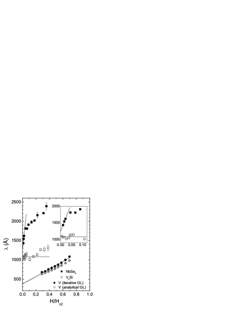
Figure 13: Magnetic field dependence of $\lambda$ determined from $\mu$SR measurements on V, V₃Si (Ref. Sonier:04 ) and NbSe₂ (Ref. Callaghan:05 ). The straight lines are linear extrapolations of the data to zero field. Inset: Blow up of the low-field data for V₃Si and NbSe₂.

The magnetic field dependence of $\lambda$ in V, as determined by both the analytical and iterative GL models, is plotted in Fig. 13, along with our previously published data for V₃Si (Ref. Sonier:04 ) and NbSe₂ (Ref. Callaghan:05 ). $\lambda$ from both models is seen to increase with field, although use of the iterative model results in a slightly stronger field dependence. The value of $\lambda$ determined by $\mu$SR depends on the radial decay of $B({\bf r})$ outside the vortex cores. Since the spatial field profile around a vortex core can be significantly modifed by the delocalization of bound core states, the measured value of $\lambda$ may be strongly dependent on field. We stress that when this is the case, $\lambda(H)$ is an “effective” length scale, which in the fits absorbs changes in $B({\bf r})$ due to changes in the electronic structure of the vortex lattice. This dominates over the weak field dependence of $\lambda$ expected for an isolated vortex in an $s$-wave superconductor.Bardeen:54 We note that the difference in slope of $\lambda$ vs $H$ between the two models in Fig. 13 suggests that the exact details of how these changes in electronic structure are absorbed by $\lambda(H)$ is model dependent. To compare with measurements of $\lambda$ by other experimental techniques, we have extrapolated the data for $\lambda(H)$ to $H\!\rightarrow\!0$ kOe. The zero-field extrapolated value of $\lambda$ in V is $376.3\!\pm\!22.4$ Å using the iterative GL model and $375.9\!\pm\!17.0$ Å using the analytical GL model. Magnetization measurementsMoser:82 ; Radebaugh:66a ; Sekula:72 have determined that $\lambda$ is in the range 374 Å to 398 Å, in excellent agreement with our results. We see that either model for $B({\bf r})$ can be used to extract a reliable measure of the zero-field magnetic penetration depth.

In V₃Si, where the bound core states are highly localized at low fields,Boaknin:03 $\lambda$ is weakly dependent on field below $H\!\approx\!0.2H_{c2}$ (Ref. Sonier:04 ). The zero-field extrapolation shown in the inset of Fig. 13 yields $\lambda\!=\!1080\!~{}\pm~{}\!17$ Å, in good agreement with the value $\lambda\!=\!1050$ Å determined from $H_{c2}(T)$ measurements in Ref. Yethiraj:05 . Likewise, the zero-field extrapolated value $\lambda=\!1249\!\pm\!31$ Å for NbSe₂ agrees well with the value of 1240 Å obtained in Ref. Finley:80 from magnetization measurements. Thus $\mu$SR can be used for accurate measurements of the absolute value of the magnetic penetration depth in type-II superconductors, provided there is sufficient data to permit an accurate extrapolation to zero field. This works even in the case of an unconventional superconductor. Recently, it was shown that zero-field extrapolated values of $\lambda$ obtained from $\mu$SR measurements on the high temperature superconductor YBa₂Cu₃O_6+x agree well with values obtained from accurate electron spin resonance measurements in the Meissner phase.Pereg:04 We note that the linear extrapolations of the data in Fig. 13 are continuous through the Meissner phase—which occurs in V below $H_{c1}\!\approx\!0.25H_{c2}$.

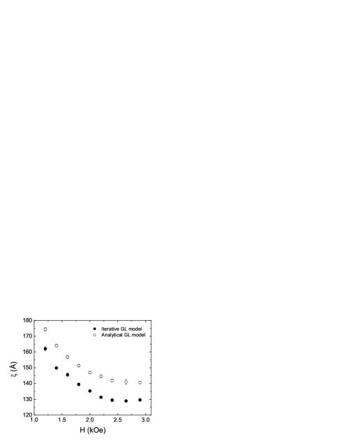
Figure 14: Magnetic field dependence of $\xi$ in V at $T\!=\!0.02$ K as determined from fits using the iterative and analytical GL models.

The magnetic field dependence of $\xi$ at $T\!=\!0.02$ K is plotted in Fig. 14. Although the analytical model yields larger values of $\xi$, both models display a similar field dependence over the entire field range. Immediately above $H_{c1}$, the vortex core size ($\sim\!\xi$) shrinks with increasing field and saturates above $H\approx 2.4$ kOe. (We note that analysis of a recent Andreev reflection spectroscopy study of niobium revealed a similar trend for $\xi(H)$ over the same range of reduced fields $0.3\leq b\leq 0.7$.Shan:06 ) We attribute this behavior to an increase in the overlap of the core states of nearest-neighbor vortices,Ichioka:99 as was found to be the case in V₃Si and NbSe₂.Sonier:04 ; Callaghan:05 Although Kogan and Zhelezina Kogan:05 have also successfully modeled the field dependence of the core size in V₃Si and NbSe₂ by weak-coupling BCS theory, their calculations assume a large GL parameter $\kappa=\lambda/\xi$ and hence are not applicable to V. In an isotropic $s$-wave superconductor, the delocalization of core states is predicted to be significant at fields above $B^{*}\!\approx\!B_{c2}/3$, although the value of this crossover field is reduced somewhat by anisotropy.Nakai:04 Specific heatRadebaugh:66a and ultrasonic attenuationBohm:63 measurements suggest that the anisotropy of the superconducting energy gap in V is approximately 10 %. According to the calculations of Ref. Nakai:04 , significant delocalization of the core states and a reduction in the core size should occur above $B^{*}\approx 1.3$ kG. Given the uncertainty in the values of $B_{c2}(T\to 0)$ and the anisotropy, the observed shrinking of the vortex cores at fields $H\geq 1.2$ kOe seems reasonable.

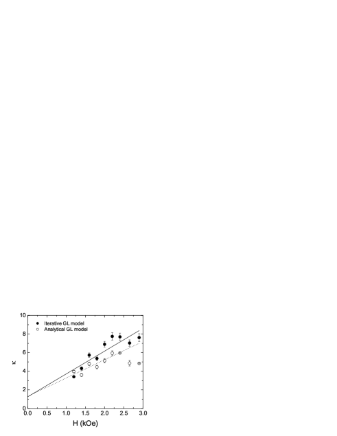
Figure 15: Magnetic field dependence of $\kappa\!=\!\lambda/\xi$ in V at $T\!=\!0.02$ K as determined from the iterative and analytical GL models. The solid (dotted) line is a linear fit to the data obtained from the iterative (analytical) GL model (see main text). The fit to the data obtained from the analytical model excludes the points at $H=2.65$ kOe and 2.9 kOe.

Finally, we present the magnetic field dependence of the GL parameter $\kappa=\lambda/\xi$ in Fig. 15. The increase in $\kappa$ with field is due to the field dependences of $\lambda$ and $\xi$. The straight lines in Fig 15 show that $\kappa$ is roughly a linear function of $H$. Significant deviations from this behavior occur for the values of $\kappa$ at the two highest fields determined from fits to the analytical GL model. This is perhaps due to the fact that the analytical model breaks down at high reduced fields $b$. It was found that both scatter and uncertainty in the values of $\lambda$ and $\xi$ were considerably reduced by fixing $\kappa$ at each field to lie on the straight line fits shown in Fig. 15. The $\xi(H)$ and $\lambda(H)$ data in Figs. 13 and 14 were obtained in this way. The zero-field extrapolated values of $\kappa$ determined from the fits shown in Fig. 15 are $1.26\pm 1.01$ for the iterative model and $1.30\pm 0.64$ for the analytical model. We note that both of these values agree well with the value $\kappa=1.34$ calculated from our estimated values of $\lambda(H=0)$ and $\xi_{0}$. Also, within experimental uncertainty, both extrapolated values of $\kappa$ are comparable with that obtained by other experimental methods for samples of similar purity.Moser:82

VI Summary and Conclusions

We have analyzed $\mu$SR measurements of the internal magnetic field distribution in the vortex state of the low-$\kappa$ type-II superconductor V using both Brandt’s iterative GL methodBrandt:97 and the analytical GL model of Ref. Yaouanc:97 . Surprisingly, the two models produce qualitatively similar results for both the temperature and field dependences of $\lambda$ and $\xi$. In particular, fits to each model yield low-temperature, zero-field extrapolated values of $\lambda$ and $\kappa$ that agree with previous measurements of these quantities by other techniques. We find that the largest difference between the results using these models occurs at high fields, where the analytical GL model is being applied outside its range of validity. The observed field dependences of $\lambda$ and $\xi$ in V are likely due to the delocalization of quasiparticle core states, as has already been established in other conventional superconductors.

We thank Prof. E. M. Forgan and Prof. E. H. Brandt for fruitful discussions and we are grateful to P. Dosanjh and K. Musselman for assistance with resistivity measurements. The work presented here was supported by the Natural Science and Engineering Research Council of Canada, and the Canadian Institute for Advanced Research. We thank staff at TRIUMF’s Centre for Molecular and Materials Science for technical assistance with the $\mu$SR experiments.

References

- (1) J.E. Sonier, J.H. Brewer, and R.F. Kiefl, Rev. Mod. Phys. 72, 769 (2000).
- (2) I.G. de Oliveira and A.M. Thompson, Phys. Rev B 57, 7477 (1998).
- (3) J.R. Clem, J. Low Temp. Phys. 18, 427 (1975).
- (4) A. Yaouanc, P. Dalmas de Réotier, and E.H. Brandt, Phys. Rev. B 55, 11107 (1997).
- (5) Z. Hao, J.R. Clem, M.W. McElfresh, L. Civale, A.P. Malozemoff, and F. Holtzberg, Phys. Rev. B 43, 2844 (1991).
- (6) W.V. Pogosov, K.I. Kugel, A.L. Rakhmanov, and E.H. Brandt, Phys. Rev. B 64, 064517 (2001).
- (7) J.E. Sonier, F.D. Callaghan, R.I. Miller, E. Boaknin, L. Taillefer, R.F. Kiefl, J.H. Brewer, K.F. Poon, and J.D. Brewer, Phys. Rev. Lett. 93, 017002 (2004).
- (8) F.D. Callaghan, M. Laulajainen, C.V. Kaiser, and J.E. Sonier, Phys. Rev. Lett. 95, 197001 (2005).
- (9) J.E. Sonier, J.H. Brewer, R.F. Kiefl, D.A. Bonn, S.R. Dunsiger, W.N. Hardy, R. Liang, W.A. MacFarlane, R.I. Miller, T.M. Riseman, D.R. Noakes, C.E. Stronach, and M.F. White, Jr., Phys. Rev. Lett. 79, 2875 (1997).
- (10) J.E. Sonier, J.H. Brewer, R.F. Kiefl, G.D. Morris, R.I. Miller, D.A. Bonn, J. Chakhalian, R.H. Heffner, W.N. Hardy, and R. Liang, Phys. Rev. Lett. 83, 4156 (1999).
- (11) E.H. Brandt, Phys. Rev. Lett. 78, 2208 (1997).
- (12) E.H. Brandt (private communication).
- (13) E.H. Brandt, J. Low Temp. Phys. 73, 355 (1988).
- (14) Goodfellow Ltd., Cambridge, UK (www.goodfellow.com).
- (15) Colin M. Hurd, The Hall Effect in Metals and Alloys (Plenum Press, 1972).
- (16) Charles Kittel, Introduction to Solid State Physics, Eighth Edition (John Wiley and Sons, 2005).
- (17) E.M. Forgan (private communication).
- (18) A. Schenck, Muon Spin Rotation Spectroscopy: Principles and Applications in Solid State Physics (Adam Hilger, Bristol, England, 1985).
- (19) V.G. Storchak and N.V. Prokof‘ev, Rev. Mod. Phys. 70, 929 (1998).
- (20) E.H. Brandt and A. Seeger, Adv. Phys. 35, 189 (1986).
- (21) E.H. Brandt, Phys. Rev. B 37, 2349(R) (1988).
- (22) B. Muhlschlegel, Z. Phys. 155, 313 (1959).
- (23) M. Tinkham, Introduction to Superconductivity, Second Edition (McGraw-Hill, 1996).
- (24) L. Kramer and W. Pesch, Z. Phys. 269, 59 (1974).
- (25) R.I. Miller, R.F. Kiefl, J.H. Brewer, J. Chakhalian, S. Dunsiger, G.D. Morris, J.E. Sonier, and W.A. MacFarlane, Phys. Rev. Lett. 85, 1540 (2000).
- (26) J.E. Sonier, J. Phys. Condens. Matter 16, S4499 (2004).
- (27) N. Hayashi, Y. Kato, and M. Sigrist, J. Low Temp. Phys. 139, 79 (2005).
- (28) N. Hayashi, T. Isoshima, M. Ichioka, and K. Machida, Phys. Rev. Lett. 80, 2921 (1998).
- (29) J.E. Sonier, R.F. Kiefl, J.H. Brewer, J. Chakhalian, S.R. Dunsiger, W.A. MacFarlane, R.I. Miller, A. Wong, G.M. Luke, and J.W. Brill, Phys. Rev. Lett. 79, 1742 (1997).
- (30) J. Bardeen, Phys. Rev. 94, 554 (1954).
- (31) E. Moser, E.Seidl, and H.W. Weber, J. Low Temp. Phys. 49, 585 (1982).
- (32) R. Radebaugh and P. H. Keesom, Phys. Rev. 149, 217 (1966).
- (33) S.T. Sekula and R.H. Kernohan, Phys. Rev. B 5, 904 (1972).
- (34) E. Boaknin, M.A. Tanatar, J. Paglione, D. Hawthorn, F. Ronning, R.W. Hill, M. Sutherland, L. Taillefer, J. Sonier, S.M. Hayden, and J.W. Brill, Phys. Rev. Lett. 90, 117003 (2003).
- (35) M. Yethiraj, D.K. Christen, A.A. Gapud, D.McK. Paul, S.J. Crowe, C.D. Dewhurst, R. Cubitt, L. Porcar, and A. Gurevich, Phys. Rev. B 72, 060504 (2005).
- (36) J.J. Finley and B.S. Deaver Jr., Solid State Commun. 36, 493 (1980).
- (37) T. Pereg-Barnea, P.J. Turner, R. Harris, G.K. Mullins, J.S. Bobowski, M. Raudsepp, R. Liang, D.A. Bonn, and W.N. Hardy, Phys. Rev. B 69, 184513 (2004).
- (38) L. Shan, Y. Huang, C. Ren, and H.H. Wen, Phys. Rev. B 73, 134508 (2006).
- (39) M. Ichioka, A. Hasegawa, and K. Machida, Phys. Rev. B 59, 184 (1999).
- (40) V.G. Kogan and N.V. Zhelezina, Phys. Rev. B 71, 134505 (2005).
- (41) N. Nakai, P. Miranović, M. Ichioka, and K. Machida, Phys. Rev. B 70, 100503(R) (2004).
- (42) H.V. Bohm and N.H. Horwitz, in Proceedings of the Eighth International Conference on Low Temperature Physics, edited by R.O. Davies (Butterworth Scientific Publications Ltd., London, 1963), p.191.