$\epsilon$ expansion for a Fermi gas at infinite scattering length

Abstract

We show that there exists a systematic expansion around four spatial dimensions for Fermi gas in the unitarity regime. We perform the calculations to leading and next-to-leading orders in the expansion over $\epsilon=4-d$, where $d$ is the dimensionality of space. We find the ratio of chemical potential and Fermi energy to be $\mu/\varepsilon_{\mathrm{F}}=\frac{1}{2}\epsilon^{3/2}+\frac{1}{16}\epsilon^{5/2}\ln\epsilon-0.0246\,\epsilon^{5/2}+\cdots$ and the ratio of the gap in the fermion quasiparticle spectrum and the chemical potential to be $\Delta/\mu=2\epsilon^{-1}-0.691+\cdots$. The minimum of the fermion dispersion curve is located at $|{\bm{p}}|=(2m\varepsilon_{0})^{1/2}$ where $\varepsilon_{0}/\mu=2+O(\epsilon)$. Extrapolation to $d=3$ gives results consistent with Monte Carlo simulations.

Introduction.— Dilute Fermi gas at infinite scattering length Leggett ; Nozieres has attracted considerable attention recently. The system can be realized in atomic traps using the Feshbach resonance OHara ; Jin ; Grimm ; Ketterle ; Thomas ; Salomon ; Thomas05 . It might be relevant for the physics of dilute neutron gas Bertsch . It has been suggested that its understanding may be important for the understanding of high-$T_{c}$ superconductivity highTc . From the theoretical perspective this is a unique nonrelativistic system that has no intrinsic scale parameter.

Theoretical treatment of the system is difficult, however, precisely due to the lack of the any small dimensionless quantity. The usual Green’s function techniques of many-body physics become completely unreliable since the expansion parameter is large, $na^{3}\gg 1$. So far, no systematic treatment has emerged. Recently considerable progress has been made by Monte Carlo simulations Carlson2003 ; Chen:2003vy ; Astrakharchik2004 ; Carlson:2005kg . However, there are many reasons that make an analytical treatment, if it exists, extremely useful. First, there are many problems that still cannot be solved by Monte Carlo simulations. Examples include polarized Fermi gases, recently realized in experiments Ketterle-polarized ; Hulet-polarized , but whose lattice realization suffers a fermion sign problem, and questions related to dynamics like the dynamical response function and the kinetic coefficients. Second, in many cases analytical approaches give unique insights that are not obvious from numerics.

In this Letter we propose an approach based on an expansion around four spatial dimensions. In this approach, one would be doing calculation in $4-\epsilon$ spatial dimensions, where the small number $\epsilon$ is used as a parameter of the perturbative expansion. Results for the physical case of three spatial dimensions are obtained by extrapolating the series expansions to $\epsilon=1$. This approach has been extremely fruitful in the theory of the second order phase transition WilsonKogut . In our case, we find that even at $\epsilon=1$ the series over $\epsilon$ is reasonably well-behaved, strongly suggesting that the limit $d\to 4$ is not only theoretically interesting but also practically useful.

The special role of four spatial dimensions has been recognized by Nussinov and Nussinov nussinov04 . They noticed that at infinite scattering length, the two-body wavefunction has a $1/r^{2}$ behavior when the separation between two fermions $r$ becomes small. The normalization integral of the wavefunction has a logarithmic singularity at $r\to 0$, from which it is concluded that at $d=4$ the system must become a noninteracting Bose gas. As far as we know, no other attempt to exploit this special property of four dimensions has been made prior to our work.

Feynman rules and the counting of the powers of $\epsilon$.— Due to the universality of the unitary Fermi gas, any short-range two-body interaction can be used, if it corresponds to the infinite scattering length. In particular, we can choose to work with the Lagrangian of local four-Fermi interaction. After a Hubbard-Stratonovich transformation, the Lagrangian density of the unitary Fermi gas can be written as (here and below $\hbar=1$)

$$\begin{split}\mathcal{L}&=\Psi^{\dagger}\left(i\partial_{t}+\frac{\sigma_{3}\bm{\nabla}^{2}}{2m}\right)\Psi+\mu\Psi^{\dagger}\sigma_{3}\Psi\\ &\qquad\qquad\quad-\frac{1}{c_{0}}\phi^{*}\phi+\Psi^{\dagger}\sigma_{+}\Psi\phi+\Psi^{\dagger}\sigma_{-}\Psi\phi^{*},\end{split}$$ (1)

where $c_{0}$ is chosen to correspond to infinite scattering length. In dimensional regularization, which we will use, $c_{0}=\infty$. From now on we set $1/c_{0}=0$. Here $\Psi$ is a two-component Nambu–Gor’kov field, $\Psi=(\psi_{\uparrow},\psi^{\dagger}_{\downarrow})^{T}$, $\sigma_{\pm}=\frac{1}{2}(\sigma_{1}\pm i\sigma_{2})$, and $\sigma_{1,2,3}$ are the Pauli matrices.

The ground state is a superfluid state where $\phi$ condenses: $\langle\phi\rangle=\phi_{0}$. We choose $\phi_{0}$ to be real. Then we expand

$$\phi=\phi_{0}+g\varphi,\qquad g=\frac{(8\pi^{2}\epsilon)^{1/2}}{m}\left(\frac{m\phi_{0}}{2\pi}\right)^{\epsilon/4},$$ (2)

where $g\sim O(\epsilon^{1/2})$ was chosen for later convenience, and rewrite the Lagrangian density as a sum: $\mathcal{L}=\mathcal{L}_{0}+\mathcal{L}_{1}+\mathcal{L}_{2}$, where

$$\begin{split}\mathcal{L}_{0}&=\Psi^{\dagger}\left(i\partial_{t}+\frac{\sigma_{3}\bm{\nabla}^{2}}{2m}+\sigma_{+}\phi_{0}+\sigma_{-}\phi_{0}\right)\Psi\\ &\qquad+\varphi^{*}\left(i\partial_{t}+\frac{\bm{\nabla}^{2}}{4m}\right)\varphi\,,\end{split}$$ (3)

$$\mathcal{L}_{1} =g\Psi^{\dagger}\sigma_{+}\Psi\varphi+g\Psi^{\dagger}\sigma_{-}\Psi\varphi^{*}+\mu\Psi^{\dagger}\sigma_{3}\Psi+2\mu\varphi^{*}\varphi\,,\phantom{\int}$$ (4)

$$\mathcal{L}_{2} =-\varphi^{*}\left(i\partial_{t}+\frac{\bm{\nabla}^{2}}{4m}\right)\varphi-2\mu\varphi^{*}\varphi\,.$$ (5)

The part $\mathcal{L}_{0}$ is a Lagrangian density of noninteracting fermion quasiparticles and a boson with mass $2m$, whose kinetic terms are introduced by hand in $\mathcal{L}_{0}$ and taken out in $\mathcal{L}_{2}$. The propagators are generated by $\mathcal{L}_{0}$ and the vertices by $\mathcal{L}_{1}$ and $\mathcal{L}_{2}$. The fermion propagator is a $2\times 2$ matrix,

$$G(p_{0},{\bm{p}})=\frac{1}{p_{0}^{2}-E_{\bm{p}}^{2}+i\delta}\left(\begin{array}[]{cc}p_{0}+\varepsilon_{\bm{p}}&-\phi_{0}\\ -\phi_{0}&p_{0}-\varepsilon_{\bm{p}}\end{array}\right),$$ (6)

where $\varepsilon_{\bm{p}}=p^{2}/2m$ and $E_{\bm{p}}=(\varepsilon_{\bm{p}}^{2}+\phi_{0}^{2})^{1/2}$. The boson propagator is

$$D(p_{0},{\bm{p}})=\left(p_{0}-\frac{\varepsilon_{\bm{p}}}{2}+i\delta\right)^{-1}.$$ (7)

The vertices come from $\mathcal{L}_{1}$ and $\mathcal{L}_{2}$ and are depicted in Fig. 1, where

$$\Pi_{0}=p_{0}-\frac{\varepsilon_{\bm{p}}}{2}.$$ (8)

The fermion-boson coupling is proportional to $g$ and is small in the limit $\epsilon\to 0$.

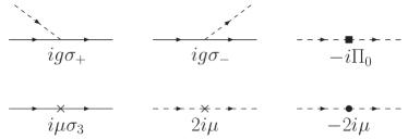
Figure 1: Feynman rules. The two vertices on the last column come from $\mathcal{L}_{2}$, while the rest from $\mathcal{L}_{1}$. Solid (dotted) lines represent the fermion (boson) propagator $iG$ $(iD)$.

Let us first consider Feynman diagrams constructed from $\mathcal{L}_{0}$ and $\mathcal{L}_{1}$ only, without the vertices from $\mathcal{L}_{2}$. We make a prior assumption $\mu/\phi_{0}\sim\epsilon$, which will be checked, and consider $\phi_{0}$ to be $O(1)$. Each pair of boson-fermion vertices brings a factor of $\epsilon$, as each $\mu$ insertion. Therefore the naive power of $\epsilon$ for a given diagram is $N_{g}/2+N_{\mu}$, where $N_{g}$ is the number of vertices and $N_{\mu}$ is the number of $\mu$ insertions. However, this naive counting does not take into account the fact that there might be inverse powers of $\epsilon$ coming from integrals which diverge at $d=4$. Using a power counting similar to that in relativistic field theories, one can show that inverse powers of $\epsilon$ appear only in diagrams with no more than three external legs. Moreover, from the analytic properties of $G(p)$ and $D(p)$ in the ultraviolet region, one can show that there are only four diagrams which have $1/\epsilon$ singularity near four dimensions. They are one-loop diagrams of the boson self-energy [Figs. 2(a) and 2(c)], $\varphi$ tadpole [Fig. 2(e)], and vacuum (the middle of Fig. 3). The diagrams in Figs. 2(a) and 2(c) combine with the vertices from $\mathcal{L}_{2}$ to restore the naive $\epsilon$ power counting.

For example, the diagram in Fig. 2(a) is

$$-i\Pi(p)=-g^{2}\int\!\frac{dk}{(2\pi)^{d+1}}\,G_{11}\!\left(k-\frac{p}{2}\right)G_{22}\!\left(k+\frac{p}{2}\right).\\$$ (9)

The integral has a pole at $d=4$, so it is $O(1)$ instead of $O(\epsilon)$ according to the naive counting. The residue at the pole can be computed as

$$\Pi(p)=-\left(p_{0}-\frac{\varepsilon_{\bm{p}}}{2}\right)+O(\epsilon),$$ (10)

which is canceled out exactly by the vertex $\Pi_{0}$ in $\mathcal{L}_{2}$. Therefore the sum of Figs. 2(a) and 2(b) is $O(\epsilon)$.

Similarly, the diagram in Fig. 2(c) contains a $1/\epsilon$ singularity, and is $O(\epsilon)$ instead of naive $O(\epsilon^{2})$. The leading part of this diagram is canceled out by the second vertex from $\mathcal{L}_{2}$, and the total is again $O(\epsilon^{2})$.

Finally, the $\varphi$ tadpole diagram with one $\mu$ insertion [Fig. 2(e)] is $O(\epsilon^{1/2})$ instead of naive $O(\epsilon^{3/2})$. The only diagram that can cancel this is the tadpole diagram with no $\mu$ insertion, Fig. 2(f). The condition of cancellation determines $\phi_{0}(\mu)$ to leading order in $\epsilon$. This condition will be automatically satisfied by the minimization of the effective potential.

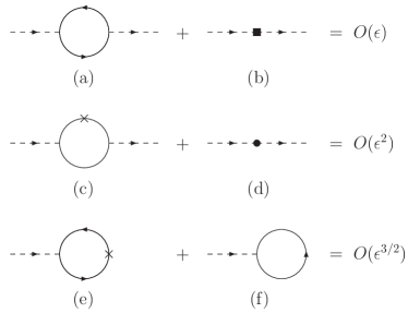
Figure 2: Restoration of naive $\epsilon$ counting for the boson self-energy and the cancellation of tadpole diagrams. The fermion loop in (c) goes around clockwise and counterclockwise.

Thus, we can now develop a diagrammatic technique for our system. For any Green’s function, we write down all Feynman diagrams according to the Feynman rules, using the propagators from $\mathcal{L}_{0}$ and the vertices from $\mathcal{L}_{1}$. If there is any subdiagram of the type in Fig. 2(a) and Fig. 2(c), we add a diagram with a vertex from $\mathcal{L}_{2}$. The result will be $O(\epsilon^{N_{g}/2+N_{\mu}})$ .

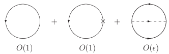
Figure 3: Vacuum diagrams for the effective potential up to next-to-leading order in $\epsilon$. The second diagram is $O(1)$ instead of naive $O(\epsilon)$ because of the $1/\epsilon$ singularity.

Leading and next-to-leading order results.— We shall perform explicit calculations, employing the Feynman rules and the $\epsilon$ power counting that have just been developed, to leading and next-to-leading orders. The dependence of $\phi_{0}$ on $\mu$ is most conveniently computed from the minimization of the effective potential $V_{\mathrm{eff}}(\phi_{0})$ Peskin:1995ev . To next-to-leading order, the effective potential receives contribution from three vacuum diagrams drawn in Fig. 3: fermion loops with and without a $\mu$ insertion and a fermion loop with the boson exchange. The contribution from the one-loop diagrams reads

$$\begin{split}V_{1}(\phi_{0})&=\frac{\phi_{0}}{3}\left[1+\frac{7-3(\gamma+\ln 2)}{6}\epsilon\right]\left(\frac{m\phi_{0}}{2\pi}\right)^{d/2}\\ &\ \ -\frac{\mu}{\epsilon}\left[1+\frac{1-2(\gamma-\ln 2)}{4}\epsilon\right]\left(\frac{m\phi_{0}}{2\pi}\right)^{d/2},\end{split}$$ (11)

where $\gamma\approx 0.57722$ is the Euler-Mascheroni constant. The contribution of the two-loop diagram is

$$V_{2}(\phi_{0}) =g^{2}\int\!\frac{dp\,dq}{(2\pi)^{2d+2}}\,G_{11}(p)G_{22}(q)D(p-q)$$ (12)

$$=-\frac{g^{2}}{4}\!\int\!\frac{d{\bm{p}}\,d{\bm{q}}}{(2\pi)^{2d}}\,\frac{(E_{\bm{p}}-\varepsilon_{\bm{p}})(E_{\bm{q}}-\varepsilon_{\bm{q}})}{E_{\bm{p}}E_{\bm{q}}(E_{\bm{p}}+E_{\bm{q}}+\varepsilon_{{\bm{p}}-{\bm{q}}}/2)}.$$

This integral is convergent even at $d=4$. Its value is

$$V_{2}(\phi_{0})=-C\epsilon\left(\frac{m\phi_{0}}{2\pi}\right)^{d/2}\phi_{0},$$ (13)

where the constant $C$ is given by a two-dimensional integral

$$\begin{split}C&=\int_{0}^{\infty}\!dx\int_{0}^{\infty}\!dy\,\frac{[f(x)-x][f(y)-y]}{f(x)f(y)}\\ &\qquad\qquad\qquad\times\left[g(x,y)-\sqrt{g^{2}(x,y)-xy}\right]\end{split}$$ (14)

with $f(x)=(x^{2}+1)^{1/2}$ and $g(x,y)=f(x)+f(y)+\frac{1}{2}(x+y)$. The result of the numerical integration is

$$C\approx 0.14424.$$ (15)

The minimum of the effective potential $V_{\mathrm{eff}}(\phi_{0})=V_{1}(\phi_{0})+V_{2}(\phi_{0})$ is located at

$$\phi_{0}=\frac{2\mu}{\epsilon}[1+(3C-1+\ln 2)\epsilon].$$ (16)

Note that the previously made assumption $\mu/\phi_{0}=O(\epsilon)$ is now checked. Also if one used the mean field approximation, one would reproduce the leading $2\mu/\epsilon$ term in Eq. (16), but not the $O(\epsilon)$ correction. The value of $V_{\mathrm{eff}}$ at $\phi_{0}$ in Eq. (16) determines the pressure $P=-V_{\mathrm{eff}}(\phi_{0})$ at chemical potential $\mu$. The density is determined from $n=\partial P/\partial\mu$, and the Fermi energy from the thermodynamic of free gas in $d$ dimensions is given by

$$\varepsilon_{\mathrm{F}}=\frac{2\pi}{m}\left[\frac{1}{2}\Gamma\left(\frac{d}{2}+1\right)n\right]^{2/d}=\frac{\phi_{0}}{\epsilon^{2/d}}\left(1-\frac{1-\ln 2}{4}\epsilon\right).$$ (17)

The nontrivial power of $\epsilon$ comes from taking $n\sim\epsilon^{-1}$ to the power of $2/d$. We find the parameter $\xi\equiv\mu/\varepsilon_{\mathrm{F}}$,

$$\xi=\frac{\epsilon^{3/2}}{2}\exp\!\left(\frac{\epsilon\ln\epsilon}{8-2\epsilon}\right)\left[1-\left(3C-\frac{5}{4}(1-\ln 2)\right)\epsilon\right].$$ (18)

Substituting the numerical value for $C$, one finds

$$\xi=\frac{1}{2}\epsilon^{3/2}+\frac{1}{16}\epsilon^{5/2}\ln\epsilon-0.0246\,\epsilon^{5/2}+\cdots.$$ (19)

The smallness of the coefficient in front of $\epsilon^{5/2}$ is a result of a cancellation between the two-loop correction and the subleading terms from the expansion of the one-loop diagrams around $d=4$.

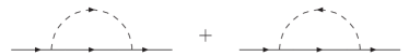
Figure 4: One-loop diagrams for the fermion self-energy of order $O(\epsilon)$.

Quasiparticle spectrum.— To leading order, the dispersion relation of fermion quasiparticles is $\omega({\bm{p}})=E_{\bm{p}}=(\varepsilon_{\bm{p}}^{2}+\phi_{0}^{2})^{1/2}$. It has a minimum at ${\bm{p}}=\bm{0}$ with a gap equal to $\Delta=\phi_{0}=2\mu/\epsilon$. The next-to-leading order correction comes from three sources: from the correction of $\phi_{0}$ in Eq. (16), from a $\mu$ insertion to the fermion propagator, and from the one-loop self-energy diagrams, $-i\Sigma(p)$, depicted in Fig. 4. Using the Feynman rules one can see that there are corrections only to the diagonal elements of the self energy:

$$\begin{split}\Sigma_{11}(p)&=ig^{2}\!\int\!\frac{dk}{(2\pi)^{d+1}}\,G_{22}(k)D(p-k)\\ &=-\frac{g^{2}}{2}\!\int\!\frac{d{\bm{k}}}{(2\pi)^{d}}\,\frac{E_{\bm{k}}-\varepsilon_{\bm{k}}}{E_{\bm{k}}(E_{\bm{k}}+\varepsilon_{{\bm{k}}-{\bm{p}}}/2-p_{0})}\end{split}$$ (20)

and $\Sigma_{22}(p_{0},{\bm{p}})=-\Sigma_{11}(-p_{0},{\bm{p}})$. To find the correction to the dispersion relation around its minimum, we only have to evaluate the self-energy at $p_{0}=\phi_{0}$, $\varepsilon_{\bm{p}}\sim\mu$ and expand $\Sigma(p_{0},{\bm{p}})=\Sigma^{0}(\phi_{0},\bm{0})+\Sigma^{\prime}(\phi_{0},\bm{0})\,\varepsilon_{\bm{p}}/\phi_{0}$. By solving the equation $\det[G^{-1}(\omega,{\bm{p}})+\mu\sigma_{3}-\Sigma(\omega,{\bm{p}})]=0$ in terms of $\omega$, we see the dispersion relation around its minimum is given by

$$\omega({\bm{p}})=\Delta+\frac{(\varepsilon_{\bm{p}}-\varepsilon_{0})^{2}}{2\phi_{0}},$$ (21)

where $\Delta=\phi_{0}+(\Sigma_{11}^{0}+\Sigma_{22}^{0})/2$ and $\varepsilon_{0}=\mu+(\Sigma_{22}^{0}-\Sigma_{11}^{0})/2-(\Sigma_{11}^{\prime}+\Sigma_{22}^{\prime})/2$.

The result of an explicit calculation is the following. The minimum of the dispersion curve is located at a nonzero value of momentum, $|{\bm{p}}|=(2m\varepsilon_{0})^{1/2}$, where

$$\varepsilon_{0}=2\mu.$$ (22)

Note the difference with the mean field approximation, in which $\varepsilon_{0}=\mu$. The correction to the gap is

$$\frac{1}{2}[\Sigma_{11}(\phi_{0},\bm{0})+\Sigma_{22}(\phi_{0},\bm{0})]=-\epsilon\left(8\ln 3-12\ln 2\right)\phi_{0}.$$ (23)

Combining it with the correction in Eq. (16), we obtain

$$\frac{\Delta}{\mu}=\frac{2}{\epsilon}\left[1+(3C-1-8\ln 3+13\ln 2)\epsilon\right]\approx\frac{2}{\epsilon}-0.691.$$ (24)

Extrapolation to $\epsilon=1$.— Although the formalism is based on the smallness of $\epsilon$, we see that even at $\epsilon=1$ the corrections are reasonably small. If we naively use only the leading and next-to-leading order results, extrapolation to $\epsilon=1$ gives for three spatial dimensions

$$\xi\approx 0.475,\qquad\frac{\varepsilon_{0}}{\mu}\approx 2,\qquad\frac{\Delta}{\mu}\approx 1.31.$$ (25)

They are reasonably close to the results of recent Monte Carlo simulations, which yield $\xi\approx 0.42$, $\varepsilon_{0}/\mu\approx 1.9$, and $\Delta/\mu\approx 1.2$ Carlson:2005kg . They are also consistent with recent experimental measurements of $\xi$, where $\xi=0.51\pm 0.04$ Thomas05 and $\xi=0.46\pm 0.05$ Hulet-polarized . Thus there is a strong indication that the $\epsilon$ expansion is useful in practice. A calculation of the $\epsilon^{2}$ corrections to these results would be extremely interesting.

Conclusion.— We have developed a systematic expansion, treating the dimensionality of space as close to four, and obtained very reasonable results. As far as we know, this is the only systematic expansion for the unitary Fermi gas at zero temperature that exists at this moment. We found that the the corrections are not too big even when extrapolated to $\epsilon=1$, which suggests that the picture of the unitary Fermi gas as a collection of weakly interacting fermionic and bosonic quasiparticles may be a useful starting point even in three spatial dimensions. There is a host of problems that can be addressed using this approach: the phase diagram of the polarized system, the structure of the superfluid vortex, finite-temperature physics, etc. It is interesting to note that the critical dimension of a superfluid-normal phase transition is also four, making weak-coupling calculations reliable at any temperature for small $\epsilon$.

Acknowledgment.— The authors thank P. Arnold, M. M. Forbes, G. Rupak, M. A. Stephanov, and A. Vuorinen for discussions. Y. N. is supported by the Japan Society for the Promotion of Science for Young Scientists. This work is supported, in part, by DOE Grant No. DE-FG02-00ER41132.

References

(1)
A. J. Leggett, in Modern Trends in the Theory of Condensed
Matter (Springer, Berlin, 1980).
(2)
P. Nozières and S. Schmitt–Rink,
J. Low Temp. Phys. 59, 195 (1985).
(3)
K. M. O’Hara et al.,
Science 298, 2179 (2002).
(4)
C. A. Regal, M. Greiner, and D. S. Jin,
Phys. Rev. Lett. 92, 040403 (2004).
(5)
M. Bartenstein et al.,
Phys. Rev. Lett. 92, 120401 (2004).
(6)
M. W. Zwierlein et al.,
Phys. Rev. Lett. 92, 120403 (2004).
(7)
J. Kinast et al.,
Phys. Rev. Lett. 92, 150402 (2004).
(8)
T. Bourdel et al.,
Phys. Rev. Lett. 93, 050401 (2004).
(9)
J. Kinast et al.,
Science 307, 1296 (2005).
(10)
G. Bertsch,
Many-Body X Challenge,
in: Proc. X Conference on Recent Progress in Many-Body Theories,
eds. R. F. Bishop et al. (World Scientific, Singapore, 2000).
(11)
See, e.g., Q. Chen, J. Stajic, S. Tan, and K. Levin,
Phys. Rep. 412, 1 (2005), and references therein.
(12)
J. Carlson, S.–Y. Chang, V. R. Pandharipande, and K. E. Schmidt,
Phys. Rev. Lett. 91, 050401 (2003);
S. Y. Chang, V. R. Pandharipande, J. Carlson, and K. E. Schmidt,
Phys. Rev. A 70, 043602 (2004).
(13)
J. W. Chen and D. B. Kaplan,
Phys. Rev. Lett. 92, 257002 (2004).
(14)
G. E. Astrakharchik, J. Boronat, J. Casulleras, and S. Giorgini,
Phys. Rev. Lett. 93, 200404 (2004).
(15)
J. Carlson and S. Reddy,
Phys. Rev. Lett. 95, 060401 (2005).
(16)
M. W. Zwierlein, A. Schirotzek, C. H. Schunck, and W. Ketterle,
Science 311, 492 (2006).
(17)
G. B. Partridge, W. Li, R. I. Kamar, Y. Liao, and R G. Hulet,
Science 311, 503 (2006).
(18) K. G. Wilson and J. Kogut,
Phys. Rep. 12, 75 (1974).
(19)
Z. Nussinov and S. Nussinov,
cond-mat/0410597.
(20)
See, e.g., M. E. Peskin and D. V. Schroeder,
An Introduction to Quantum Field Theory
(Addison-Wesley, Reading MA, 1995), Sec. 11.3.