Bell Rate Model with Dynamic Disorder: Model and Its Application in the Receptor-ligand Forced Dissociation Experiments

Abstract

We extend the Bell forced dissociation rate model to take account into dynamic disorder. The motivation of the present work is from the recent forced dissociation experiments of the adhesive receptor-ligand complexes, in which some complexes were found to increase their mean lifetimes (catch bonds) when they are stretched by mechanical force, while the force increases beyond some thresholds their lifetimes decrease (slip bonds). Different from our previous model of force modulating dynamic disorder, in present work we allow that the projection of force onto the direction from the bound to the transition state of complex could be negative. Our quantitative description is based on a one-dimension diffusion-assisted reaction model. We find that, although the model can well describe the catch-slip transitions observed in the single bond P-selctin glycoprotein ligand 1(PSGL-1)$-$P- and L-selectin forced dissociation experiments, it might be physically unacceptable because the model predicts a slip-catch bond transitions when the conformational diffusion coefficient tends to zero.

I Introduction

Traditionally, the forced dissociation rate of noncovalent biological receptor-ligand bonds is described by the simple Bell expression Bell

$$k_{\rm off}(f)=k^{0}_{\rm off}\exp(f\xi^{{\ddagger}}/k_{\rm B}T),$$ (1)

where

$$k^{0}_{\rm off}=k_{0}\exp(-\Delta G^{\ddagger}/k_{\rm B}T)$$ (2)

is the intrinsic rate constant in the absence of force, $\Delta G^{\ddagger}$ is the height of the intrinsic energy barrier, $\xi^{{\ddagger}}$ is a projection of the distance from the bound state to the energy barrier onto external applied force $f$, $k_{\rm B}$ is the Boltzmann’s constant, and $T$ is absolute temperature. Bell phenomenologically introduced this expression from the kinetic theory of the strength of solids in his seminal paper more than twenty years ago. Evans and Ritchie Evans97 later put the Bell expression onto a firm theoretical bases: the bond rupture was modelled in the framework of Kramers theory as thermally assisted escape over one or several transition state barriers. The validity of the expression has been demonstrated in experiments Alon ; Chen . In the Bell forced dissociation rate model, the parameters including the energy barrier $\Delta G^{\ddagger}$ and the projection distance $\xi^{\ddagger}$ are deterministic and time independent.

On the other hand, we have known that in a large variety of chemical and physical areas, association/dissociation processes could be stochastic and time dependent. Such processes have been termed as “rate processes with dynamical disorder” in an excellent review given by Zwanzig Zwanzig in fifteen years ago. The typical examples include cyclization of polymer chains in solutions Wilemski , ligands rebinding to heme proteins Agmon , electron transfer reactions Sumi , electronic relaxation in solutions in the absence of an activation barrier Bagchi , and etc. Hence, in principle we could expect that dynamic disorder may also arise in some forced biological bond rupture experiments. But it was not until recently that we liuf1 ; liuf2 firstly pointed that this disorder might play key role in a forced dissociation experiment of the adhesive bond forming between P-selectin and P-selectin glycoprotein ligand 1 (PSGL-1) using atomic force microscopy (AFM) Marshall , though this experiment was published three years ago. A counterintuitive observation has been found: in contrast to ordinary biological bonds, the mean lifetimes of the PSGL-1$-$P-selectin bond first increase with initial application of a small force, which were termed “catch” by Dembo Dembo early, and subsequently decrease, which were termed “slip”.

The main point of the questions of dynamic disorder is that the rate coefficient depends on stochastic control variables and is fluctuating in time Zwanzig . Correspondingly, we suggested that the Bell parameters in Eq. 1 were stochastic liuf1 ; liuf2 . As one type of noncovalent bonds, interactions of adhesive receptor and their ligand is always weaker. Moreover, the interface between them has been reported to be broad and shallow, such that revealed by the crystal structure of the PSGL-1$-$P-selectin bond Somers . Therefore it is plausible that the energy barriers $\Delta G^{\ddagger}$ or the projection distance $\xi^{\ddagger}$ for the bond are fluctuating with time due to either the global conformational change or the local conformational change at the interface. Two possible cases were discussed. In the Gaussian stochastic rate model (GSRM) liuf1 , we simply assumed that $\xi^{\ddagger}$ and $\Delta G^{\ddagger}$ had basic properties of random variables. We concluded that the catch behavior of some biological adhesive bonds could arise from the stronger positive correlation between the two stochastic variables. Although the model accounted for the catch-slip bond transition in a direct and analytic way, it also predicted that the mean lifetime of the PSGL-1$-$P-selectin bond was symmetric relative to a critical force $f_{c}$, while the experimental data were clearly skewed towards a large force. In addition, the physical justice of the assumption of a stationary dissociation process may be doubtful. To overcome these shortages, we proposed an alternative and more “microscopic” model liuf2 , in which external applied force not only presents in the Bell expression, but also modulates the distribution of a “inner” conformational coordinate. We named it as force modulating dynamic disorder (FMDD) model in the following. In contrast to the GSRM, we only allowed the energy barrier to be stochastic. The quantitative description was based on a one-dimension diffusion-reaction equation Agmon . We found that agreement between our calculation and the data was impressive. This model also suggests a new physical explanation of the catch-slip bond: the transition could arise from a competition of the two components of applied force along the directions of the dissociation reaction coordinate and the complex conformational coordinate; the former accelerates the dissociation by lowering the height of the energy barrier, i.e., the slip behavior, while the later stabilizes the complex by dragging the system to the higher barrier height, i.e., the catch behavior.

Even there are apparent advantages of the FMDD model, we cannot completely exclude the GSRM, because compared to the former, the GSRM does not require that force acts on the “inner” conformation coordinate. This requirement makes us to conclude that catch-slip bond transitions would be altered by the orientation of external forces liuf2 . Although such a prediction has a potential to account for the bulk experimental observations McEver that the optimal binding of P-selectin is critically dependent on the relative orientations of its ligand, there is no such evidence in the existing data measured by the single molecular techniques Marshall ; Evans2004 . On the other hand, we have viewed the conformational coordinate to be molecular extension which is coupled to external applied force. We also have no strong experimental evidence to support this assumption. The inner coordinate has been thought to be experimentally unaccessible. In addition, the FMDD model did not investigate the possibility of a fluctuating projection distance. In the present work, we try to give a model that force does not modulate the conformational coordinate of the complex while presenting catch-slip behaviors simultaneously. Our model still bases on a diffusion-reaction equation. Different from the FMDD model, the projective distance $\xi^{\ddagger}$ is allowed to be fluctuating and negative. Our calculation shows that this new Bell rate model with dynamic disorder not only derives the same expression of the mean lifetime which has been obtained in the GSRM before if both $\Delta G^{\ddagger}$ and $\xi^{\ddagger}$ are simple linear functions of the conformational coordinate, but also well fits to the experimental data if a slightly complicated piecewise function with two segments is used. An unexpected consequence of this model is that the transition from catch to slip converts into slip-catch transition when the conformational diffusion is “frozen” by lowering the diffusion coefficient to zero. Interestingly, the FMDD model does not predict such a conversion. Therefore, our discussion here would be useful to design new experiments to distinguish which model is physically correct.

The organization of the paper is as follows. In Sec II, we describe the physical picture of the Bell rate model with dynamic disorder and give the essential mathematic derivations. According to the value of the diffusion coefficient, we distinguish three cases: $D\to\infty$, $D\to 0$, and the intermediate $D$. Analytical solutions can be obtained for the first two cases, while for the last one we resort to numerical approach. In the following section, we study two extended Bell models at the three different coefficients, in which the barrier height and projection distance are linear and piecewise functions of the conformational coordinate, respectively. A comparison between model and the experiments is also performed. Finally we give our conclusion in Sec IV.

II Bell rate model with dynamic disorder

The physical picture of our model for the forced dissociation of the receptor-ligand bonds is very similar with the small ligand binding to heme proteins Agmon : there is a energy surface for the dissociation which dependents on both the dissociation reaction coordinate of the receptor-ligand bond and the conformational coordinate $x$ of complex, while the later is perpendicular to the former; for each complex conformation $x$ there is a different dissociation rate constant which obeys the Bell expression $k_{\rm off}(x,f)$. Higher temperature or larger diffusivity (low viscosities) allows $x$ variation within the complex to take place. Conversely, at very low temperatures (or high viscosities) the coordinate is frozen so that the complex is ruptured with the rate constant $k_{\rm off}(x,f)$ without changing their $x$ value during dissociation.

II.1 Rapid diffusion

The constant force mode. There are two types of force loading modes. First we consider the constant force case Marshall ; Sarangapani . A diffusion equation in the presence of a coordinate dependent reaction is given by Agmon

$$\frac{\partial p(x,t)}{\partial t}=D\frac{\partial^{2}p}{\partial x^{2}}+\frac{D}{k_{\rm B}T}\frac{\partial}{\partial x}\left(p\frac{\partial V}{\partial x}\right)-k_{\rm off}(x,f)p,$$ (3)

where $p(x,t)$ is the probability density for finding a value $x$ at time $t$, at initial time $p(x,0)$ is thought to be thermal equilibrium under a potential $V(x)$ without reaction, and $D$ is a constant diffusion coefficient. The motion is under influence of a potential $V(x)$ and a coordinate dependent Bell expression $k_{\rm off}(x,f)$. Because the above equation in fact is almost same with that proposed by Agmon and Hopfield except that the rate constant is controlled by applied force $f$, we only present essential mathematic derivations. More detailed discussion about the diffusion-reaction equation could be found in their original work.

Following Agmon and Hopfield Agmon , we substitute

$$p(x,t)=N_{0}\phi(x,t)\exp\left[-V(x)/2k_{\rm B}T\right]$$ (4)

into Eq. 3, one can convert the Eq. 3 into the Schr$\ddot{o}$dinger-like presentation,

$$\frac{\partial\phi}{\partial t}=D\frac{\partial^{2}\phi}{\partial x^{2}}-U_{f}(x)\phi=-{\cal H}_{f}(\phi),$$ (5)

where $N_{0}$ is the normalization constant of the density function at $t=0$, and the “effective” potential

$$U_{f}(x) = U(x)+k_{\rm off}(x,f)$$

$$= \frac{D}{2k_{\rm B}T}\left[\frac{1}{2k_{\rm B}T}\left(\frac{dV}{dx}\right)^{2}-\frac{d^{2}V}{dx^{2}}\right]+k_{\rm off}(x,f).$$

We define $U(x)$ for it is independent of the force. In principle Eq. 5 could be solved by eigenvalue technique Agmon . Particularly, at larger $D$ only the smallest eigenvalue $\lambda_{0}(f)$ mainly contributes to the eigenvalue expansion. For any given $k_{\rm off}(x,f)$, such as the exponential form in the Bell expression, there is no analytical $\lambda_{0}(f)$; instead a perturbation approach has to be applied Messiah . If the eigenfunctions and eigenvalues of the “unperturbed” Schr$\ddot{o}$dinger operator,

$${\cal H}=-D\frac{\partial^{2}}{\partial x^{2}}+U(x),$$ (7)

in the absence of $k_{\rm off}(x,f)$ have been known to be

$${\cal H}\phi^{0}_{n}=-\lambda^{0}_{n}\phi^{0}_{n},$$ (8)

and the Bell rate is adequately small (compared to the diffusion coefficient $D$), the first eigenfunction $\phi_{0}(f)$ and eigenvalue $\lambda_{0}(f)$ of the operator ${\cal H}_{f}$ then are given by

$$\phi_{0}(f) = \phi^{(0)}_{0}+\phi^{(1)}_{0}(f)+\cdots$$

$$= \phi^{0}_{0}+\sum_{m\neq 0}\frac{\int\phi^{0}_{0}(x)k_{\rm off}(x,f)\phi^{0}_{m}(x)dx}{\lambda^{0}_{0}-\lambda^{0}_{m}}\phi^{0}_{m}+\cdots$$

and

$$\lambda_{0}(f) = \lambda^{(0)}_{0}+\lambda^{(1)}_{0}(f)+\lambda^{(2)}_{0}(f)+\cdots$$

$$= \lambda^{0}_{0}+\int\phi^{0}_{0}(x)k_{\rm off}(x,f)\phi^{0}_{0}(x)dx+$$

$$\sum_{m\neq 0}\frac{\left(\int\phi^{0}_{0}(x)k_{\rm off}(x,f)\phi^{m}_{0}(x)dx\right)^{2}}{\lambda^{0}_{0}-\lambda^{0}_{m}}+\cdots,$$

respectively. Because the system is assumed to be thermal equilibrium at $t=0$, the first eigenvalue $\lambda^{0}_{0}$ must vanish. On the other hand, considering that

$$\phi_{0}^{0}(x)\propto\exp\left[-V(x)/2k_{\rm B}T\right],$$ (11)

and the square of $\phi_{0}^{0}$ is just the equilibrium Boltzmann distribution $p_{\rm eq}(x)$ under the potential $V(x)$, we rewrite the first correction of $\lambda_{0}(f)$ as

$$\lambda^{(1)}_{0}(f)=\int p_{\rm eq}(x)k_{\rm off}(x,f)dx,$$ (12)

$$p_{\rm eq}(x)\propto\exp\left[-V(x)/k_{\rm B}T\right].$$ (13)

Substituting the above formulaes to Eq. 4, the probability density function then is approximated to be

$$p(x,t)\approx N_{0}\exp\left(-\frac{V}{2k_{\rm B}T}\right)\exp[-\lambda_{0}(f)t]\phi_{0}(f).$$ (14)

The quantity measured in the constant force experiments usually is the mean lifetime of the bond,

$$\langle\tau\rangle(f)=-\int_{0}^{\infty}t\frac{dQ}{dt}dt=\int_{0}^{\infty}Q(t)dt,$$ (15)

where the survival probability $Q(t)$ is related to the probability density as

$$Q(t) = \int p(x,t)dx$$ (16)

$$\approx \exp\left[-t\left(\lambda_{0}^{(1)}(f)+\cdots\right)\right].$$

Therefore the decay of $Q(t)$ is almost a monoexponential in large $D$ limits.

The dynamic force mode. In addition to the constant force mode, force could be dynamic, e.g., force increasing with a constant loading rate in the biomembrane force probe (BFP) experiment Evans2004 . This scenario should be more complicated than that for the constant force case. We still use Eq. 3 to describe the bond dissociations by a dynamic force but the constant force therein is replaced by a time-dependent function $f_{t}$. The initial condition is the same as before. We firstly convert the diffusion-reaction equation into the Schr$\ddot{o}$dinger-like presentation again,

$$\frac{\partial\phi}{\partial t} = {\cal H}_{f_{t}}\phi$$ (17)

$$= -\left({\cal H}+k_{\rm off}(x,f_{t})\right)\phi.$$

Please note that now we face a time-dependent Sch$\ddot{o}$dinger operator, ${\cal H}_{f_{t}}$.

We know that solving a Sch$\ddot{o}$dinger equation with a time-dependent Hamiltonian is difficult. The most simplest situation is to use an adiabatic approximation analogous to what is done in quantum mechanics. Hence we immediately have Messiah

$$\phi(x,t)\approx\exp\left[-\int_{0}^{t}\left(\lambda_{0}(f_{t^{\prime}})+B(t^{\prime})\right)dt^{\prime}\right]\phi_{0}(f_{t}),$$ (18)

where the “Berry phase”,

$$B(t)=\int\phi_{0}(f_{t})\frac{\partial}{\partial t}\phi_{0}(f_{t})dx,$$ (19)

and $\phi_{0}(f_{t})$ is the first eigenfunction of ${\cal H}_{f_{t}}$. We are not very sure whether the assumption is reasonable or not in practice. But one of tests is to see the agreement between the calculation and data. We apply the perturbation approach again to obtain the eigenvalues and eigenfunctions of the time-dependent operator. Hence, we have $\phi_{0}(f_{t})$ and $\lambda_{0}(f_{t})$ by only replacing the Bell expression in Eqs. II.1 and II.1 with $k_{\rm off}(x,f_{t})$. The Berry phase then is approximated to

$$B(f_{t}) \approx \sum_{m\neq 0}\left(\frac{1}{\lambda^{0}_{m}}\right)^{2}\int\phi^{0}_{0}(x)k_{\rm off}(x,f_{t})\phi^{0}_{m}(x)dx\times$$ (20)

$$\int\phi^{0}_{0}(x)\frac{dk_{\rm off}}{dt}\phi^{0}_{m}(x)dx.$$

Finally, the survival probability for the dynamic force is given by

$$Q(t)\approx\exp\left[-\int_{0}^{t}\left(\lambda^{(1)}_{0}(f_{t^{\prime}})+B(f_{t^{\prime}})+\cdots\right)dt^{\prime}\right].$$

Different from the constant force mode, the data of the dynamic force experiments are typically presented in terms of the force histogram, which corresponds to the probability density of the dissociation forces $p(f)$

$$p(f)=-\frac{dQ}{dt}\left/\frac{df}{dt}\right.$$ (22)

Particularly, when force is a linear function of time $f=f_{0}+rt$, where $r$ is loading rate, and zero or nonzero of $f_{0}$ respectively corresponds to the steady- or jump-ramp force mode Evans2004 , we have

$$P(f,f_{0})\approx\frac{1}{r}\left[\lambda^{(1)}_{0}(f)+B(f)+\cdots\right]\times$$ (23)

$$\exp\left[-\frac{1}{r}\int_{f_{0}}^{f}\left(\lambda^{(1)}_{0}(f^{\prime})+B(f^{\prime})+\cdots\right)df^{\prime}\right].$$

II.2 Slow diffusion

At lower temperatures (or higher viscosities) the conformational coordinate is, or the diffusion coefficient $D\to 0$. In this limit, the solution of Eq. 3 for the constant force mode is simply given by

$$p(x,t)=p_{\rm eq}(x)\exp\left[-k_{\rm off}(x,f)t\right].$$ (24)

Compared to the density at larger diffusivity, the probability density in this limit closely depends on the initial distribution. Consequently, the survival probability $Q(t)$ as an integral of $p(x,t)$ is a multiexponential decay which is remarkably distinct from the monoexponential decay at larger $D$ limitation (Eq. 16). The mean lifetime of bond is given as

$$\langle\tau\rangle(f)=\int dxp_{\rm eq}(x)k^{-1}_{\rm off}(x,f).$$ (25)

For the dynamic force mode, the probability density is very simple,

$$p(x,t)=p_{\rm eq}(x)\exp\left[-\int_{0}^{t}k_{\rm off}(x,f_{t^{\prime}})dt^{\prime}\right],$$ (26)

and the probability density of the dissociation force for the ramping force at the slower diffusion is

$$P(f,f_{0}) = \int dxp_{\rm eq}(x)\frac{1}{r}k_{\rm off}(x,f)\times$$ (27)

$$\exp\left[-\frac{1}{r}\int_{f_{0}}^{f}k_{\rm off}(x,f^{\prime})df^{\prime}\right].$$

When the diffusion coefficients are between the two limiting cases, in general there are not analytical solutions to Eq. 3. We have to employ numerical approach (SSDP ver. 2.6) Krissinel .

III Two typical examples

In the present work, we only consider the bound diffusions in a harmonic potential

$$V(x)=\frac{k_{x}}{2}x^{2},$$ (28)

where $k_{x}$ is the spring constant. $\cal H$ then reduces to a harmonic oscillator operator with an effective potential

$$U(x)=\frac{Dk_{x}}{2k_{\rm B}T}\left(\frac{k_{x}x^{2}}{2k_{\rm B}T}-1\right).$$ (29)

Its eigenvalues and eigenfunctions are

$$\lambda^{0}_{n} = nDk_{x}/k_{\rm B}T$$ (30)

and

$$\phi^{0}_{n}(y) = 2^{-n/2}\pi^{-1/4}(n!)^{-1/2}e^{-z^{2}/2}H_{n}(y),$$ (31)

respectively, where $y=(k_{x}/2k_{\rm B}T)^{1/2}x$, and $H_{n}(y)$ is the Hermite polynormials Messiah . In principle, we can construct various functions of the barrier heights and projection distances with respect to the conformational coordinate $x$. In the present work, we only study the two examples, the linear functions and the piecewise functions with two segments. The former should be the simplest functional dependence on the coordinate. While the later is complex enough to compare with the real data.

III.1 Rapid diffusion limit: $D\to\infty$

Linear $\Delta G^{\ddagger}$ and $\xi^{\ddagger}$. In this limit, the higher order corrections $\lambda_{0}^{(n)},(n\geq 2)$ are negligible, and the survival probability of bond, Eq. 16, is monoexponential decay. Consequently, the mean lifetime of a bond is simply $\langle\tau\rangle(f)=1/\lambda^{(1)}_{0}(f)$. We start from the case that $\Delta G^{\ddagger}$ and $\xi^{\ddagger}$ are linear functions of the conformational coordinate,

$$\Delta G^{\ddagger}(x) = \Delta G^{\ddagger}_{0}+k_{g}x,$$

$$\xi^{\ddagger}(x) = \xi^{\ddagger}_{0}+k_{\xi}x.$$ (32)

Substituting the above equations and the harmonic potential into Eq. 12, we have

$$\lambda_{0}(f) = k_{0}\exp\left[-\beta\Delta G^{\ddagger}_{0}+\frac{\beta}{2}\frac{k_{g}^{2}}{k_{x}}-\frac{\beta k_{x}}{2k_{\xi}^{2}}\left(\frac{k_{g}k_{\xi}}{k_{x}}-\xi^{\ddagger}_{0}\right)^{2}\right]$$ (33)

$$\times\exp\left[\frac{\beta k_{\xi}^{2}}{2k_{x}}\left(f-\frac{k_{g}k_{\xi}/k_{x}-\xi^{\ddagger}_{0}}{k_{\xi}^{2}/k_{x}}\right)^{2}\right],$$

where $\beta=1/k_{\rm B}T$. We rewrite the above equation into a more compact form,

$$\lambda_{0}(f) = k_{0}\exp\left[-\beta\Delta G^{{\ddagger}}_{0}+\frac{\beta^{2}}{2}K_{g}-\frac{(\xi^{{\ddagger}}_{0}-\beta K_{g\xi})^{2}}{2K_{x}}\right]$$ (34)

$$\times\exp\left[\frac{\beta^{2}K_{\xi}}{2}\left(f-\frac{\beta K_{g\xi}-\xi^{{\ddagger}}_{0}}{\beta K_{\xi}}\right)^{2}\right],$$

by defining new variables as following,

$$K_{\xi}=\frac{k_{\xi}^{2}}{\beta k_{x}},\text{ }K_{g}=\frac{k_{g}^{2}}{\beta k_{x}},\text{ }K_{g\xi}=\frac{k_{\xi}k_{g}}{\beta k_{x}}.$$ (35)

Eq. 34 has the same expression with the average dissociation rate formally obtained in the GSRM (Eq. 6 in Ref. liuf1 and $x^{\ddagger}_{0}$ instead of $\xi^{\ddagger}_{0}$ used therein). Consequently, $K_{g}$, $K_{\xi}$ and $K_{g\xi}$ could be viewed as the variances and covariance of and between the two stochastic variables $\Delta G^{\ddagger}$ and $\xi^{\ddagger}$ at the same time point. Interestingly, it also means that we cannot get the absolute value of the parameters $k_{x}$, $k_{g}$ and $k_{\xi}$ by observing the force dependence of the dissociation rates. Although the above equation is not new, there are still several points deserving to be presented. Firstly, the derivation of Eq. 34 does not require the forced bond dissociation process stationary as the GSRM assumed. Then the correlation coefficient of the two stochastic variables is only 1 or $-1$ according to whether $k_{g}$ and $k_{\xi}$ have the same signs or not, whereas in the GSRM the coefficient is arbitrary. It is expected because both $\Delta G^{\ddagger}$ and $\xi^{\ddagger}$ here are the linear functions of the same coordinate. Finally, $\xi^{\ddagger}_{0}$ could be minus. We are not ready to discuss the general behaviors of Eq. 34 in detail because it has been performed in the GSRM. We only emphasize that the rate indeed exhibits the catch-slip bond transitions, when the following conditions hold: both the distance and the barrier height are stochastic variables, and $\xi^{\ddagger}_{\rm c}=\beta K_{g\xi}-\xi^{{\ddagger}}_{0}>0$. Because the force is always positive, the rate then will firstly decreases with the increasing of the force, and then increases when the force is beyond a threshold, $f_{\rm c}=\xi^{\ddagger}_{\rm c}/\beta K_{\xi}$. We define the new parameters $\xi^{\ddagger}_{\rm c}$ and $f_{\rm c}$ since they have the same dimensions of distance and force.

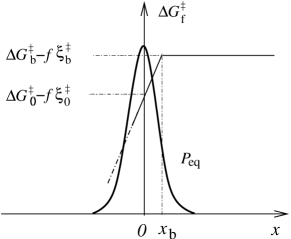
Figure 1: Schematic diagram of the piecewise functions $\Delta G^{\ddagger}_{\rm f}=\Delta G^{\ddagger}(x)-f\xi^{\ddagger}(x)$ with respect to the coordinate $x$ at a given force $f$. The symmetric curve represents the thermal equilibrium distribution of the conformational coordinate under the harmonic potential $V(x)$.

Following the GSRM, we combine the six parameters in Eq. 34 into only three: the threshold $f_{\rm c}$, the variance $K_{\xi}$, and a prefactor $N$ which is defined as

$$N=k_{0}\exp{\left[-\beta\Delta G^{{\ddagger}}_{0}+\frac{\beta^{2}}{2}K_{g}-\frac{\beta^{2}}{2}K_{\xi}(f-f_{c})^{2}\right]}$$ (36)

Then the mean lifetime has a Gaussian-like function with respect to force,

$$\langle\tau\rangle(f) = N^{-1}\exp\left[-\frac{\beta^{2}}{2}K_{\xi}(f-f_{c})^{2}\right].$$ (37)

We respectively fit the data of the forced dissociations of the single PSGL-1$-$P- Marshall and L-selectins Sarangapani bonds. The fitting results and the parameters will be showed in the next section. Because the Gaussian-like expression is symmetric relative to the threshold $f_{\rm c}$, and it is clearly inconsistent with the experimental observations, in the following section, we study a slightly complicated case.

Piecewise $\Delta G^{\ddagger}$ and $\xi^{\ddagger}$ functions. Compared to the former, the current case should be more useful because it describes the experiments better. We assume that both the barrier and distance are piecewise function with two segments: for $x\leq x_{b}$, they follow Eq. III.1; otherwise,

$$\Delta G^{\ddagger}(x) = \Delta G^{\ddagger}_{b}=\Delta G^{\ddagger}(x_{b}),$$

$$\xi^{\ddagger}(x) = \xi^{\ddagger}_{b}=\xi^{\ddagger}(x_{b}).$$ (38)

Fig. 1 is the schematic diagram of the function $\Delta G^{\ddagger}(x)-f\xi^{\ddagger}(x)$ at a given force. Substituting the functions into Eq. 12, we have

$$\lambda_{0}(f) = \frac{k_{0}}{2}\exp\left[-\beta\Delta G_{0}^{\ddagger}+\frac{\beta k_{g}^{2}}{2k_{x}}-\frac{\beta k_{x}}{2k_{\xi}^{2}}\left(\frac{k_{\xi}k_{g}}{k_{x}}-\xi_{0}^{\ddagger}\right)^{2}\right]$$

$$\times\exp\left[\frac{\beta k_{\xi}^{2}}{2k_{x}}\left(f-\frac{k_{g}k_{\xi}/k_{x}-\xi^{\ddagger}_{0}}{k_{\xi}^{2}/k_{x}}\right)^{2}\right]\times$$

$${\rm erfc}\left[-\sqrt{\frac{\beta k_{x}}{2}}\left(x_{b}+\frac{k_{g}}{k_{x}}-\frac{k_{\xi}}{k_{x}}f\right)\right]+$$

$$\frac{k_{0}}{2}\exp\left[-\beta\Delta G^{\ddagger}_{b}+\beta f\xi^{\ddagger}_{b}\right]\times{\rm erfc}\left[\sqrt{\frac{\beta k_{x}}{2}}x_{b}\right]\$$

where the complementary error function is

$${\rm erfc}(x)=\frac{2}{\sqrt{\pi}}\int_{x}^{\infty}e^{-x^{2}}dx.$$ (40)

Although the above rate expression seems to be more complex than that in the case of the linear functions, it is really a simple weighted sum of Eq. 33 and the standard Bell expression, Eq. 1. This function would yield the major characteristics of the catch-slip bond transitions if we assumed that $k_{\xi}>0$, $\xi^{\ddagger}_{b}>0$, and $k_{x}x_{b}^{2}\gg 0$: (i) if force is smaller, Eq. III.1 reduces to Eq. 33 because the asymptotic behaviors of the error function are

$${\rm erfc}(-\infty)=2,\qquad{\rm erfc}(+\infty)=0,$$ (41)

respectively; (ii) if force is larger enough, according the asymptotic expansion of the error function for large positive $x$,

$${\rm erfc}(x)\approx\frac{e^{-x^{2}}}{\sqrt{\pi}}\left(\frac{1}{x}-\frac{1}{2x^{3}}+\cdots\right),$$ (42)

it is easy to prove that Eq. III.1 tends to the standard Bell expression with a positive projection distance. This behavior has been observed in experiment Alon early. To fit the data, we rewrite Eq. III.1 into

$$\lambda_{0}(f) = \kappa_{0}\times\left\{\right.$$

$$\exp\left[\frac{\beta^{2}K_{g}}{2}-\frac{\beta^{2}K_{\xi}}{2}f_{c}^{2}\right]\times\exp\left[\frac{\beta^{2}K_{\xi}}{2}(f-f_{c})^{2}\right]$$

$$\times{\rm erfc}\left[-X_{b}-\sqrt{\frac{\beta^{2}K_{g}}{2}}+\sqrt{\frac{\beta^{2}K_{\xi}}{2}}f\right]+$$

$$\exp\left[-2X_{b}\sqrt{\frac{\beta^{2}K_{g}}{2}}+f\left(\beta^{2}K_{g\xi}^{2}-\right.\right.$$

$$\left.\left.\left.\beta^{2}K_{\xi}f_{c}+2X_{b}\sqrt{\frac{\beta^{2}K_{\xi}}{2}}\right)\right]\times{\rm erfc}[X_{b}]\right\},$$

by introducing additional definitions,

$$X_{b} = x_{b}\sqrt{\frac{\beta k_{x}}{2}},\text{ }\kappa_{0}=\frac{k_{0}}{2}\exp\left(-\beta\Delta G_{0}^{\ddagger}\right),$$ (43)

where we have replaced $\Delta G^{\ddagger}_{b}$ and $\xi^{\ddagger}_{b}$ by the linear functions. We see that we cannot determine parameters $k_{x}$, $k_{g}$ and $k_{\xi}$ by fitting the forced dissociation experiments. Totally there are five parameters presenting in the current model, $K_{\xi},\text{ }K_{g},\text{ }X_{b},\text{ }\kappa_{0}$, and $f_{c}$. In practice, we further reduce the model to the simplest case by assuming $X_{b}=0$. The fitting curves for the forced dissociations of PSGL-1$-$P-selectin and -L-selectin complex are showed in Fig. 2. We see that the agreement between the model and the data is quite good.

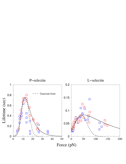
Figure 2: The mean lifetime vs. force for the bonds of dimeric P-selectin and L-selectin with the monomeric sPSGL-1 (the square) Marshall and the dimeric PSGL-1 (the circle). The reader is reminded that the data for the dimeric PSGL-1$-$P-selectin bonds has been rescaled to single bond case Pereverzev . The solid lines are the results of Eq. III.1, where the parameters are as follows: for P(L)-selectin case, $\kappa_{0}\approx 0.09$ (4.60) s^-1, $K_{g}\approx 18.5$ (3.39) ${k_{\rm B}T}^{2}$, $K_{\xi}\approx 2.0$ (0.06) nm², and $f_{\rm c}=11.0$ (27.7) pN. While the dashed lines are from the Gaussian-like Eq. 34, where the parameters are as follows: for P(L)-selectin case, $N\approx 0.76$ (0.085) s^-1, $K_{\xi}\approx 1.0$ (0.03) nm², and $f_{\rm c}\approx 12.3$ (40.0) pN. Compared to the mean lifetime vs. force in the FMDD model, the present curve decays slowly after the transition.

More challenging experiments to our theory are the force steady- and jump-ramp modes Evans2004 . In $D\to\infty$ limit, Eq. 23 reduces to

$$P(f,f_{0})=\frac{\lambda_{0}(f)}{r}\exp\left[-\frac{1}{r}\int_{f_{0}}^{f}\lambda_{0}(f^{\prime})df^{\prime}\right].$$ (44)

According Eq. 44, the probability density of dissociation force is uniquely determined by the rate $\lambda_{0}(f)$. Because both the present work and FMDD model describe the same group of experiments, here we are not ready to discuss the general characteristics of $P(f,f_{0})$; they have been done in FMDD liuf2 . When we test Eq. 44 with the parameters obtained from the constant force data, it apparently deviates from the dynamic force data Evans2004 . It must emphasize that the experiments of the constant and dynamic force modes were performed by the same experimental group and the same single bond sPSGL-1$-$P-selectin. Similar problem has been met in our previous FMDD model and two-pathway and one well model Pereverzev . We liuf2 argued and suggested that the experiment of dynamic force modes really measured the histogram of the dissociation force of the dimeric bond PSGL-1$-$P-selectin complex instead of single bond case: the two independent bonds share the same force and fail randomly. We still make use of this assumption in the present work. It is easy to relate the probability density of the dissociation force for the dimeric bonds, $P_{\rm d}(f,f_{0})$, to the single one by

$$P_{\rm d}(f,f_{0})=P\left(f/2,f_{0}/2\right)^{2}.$$ (45)

Fig. 3 is the finally result.

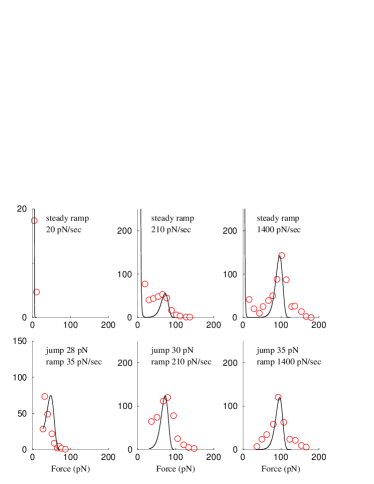
Figure 3: The probability density of the dissociation forces $P_{\rm d}(f,f_{0})$ under the different loading rates predicted by our theory (solid curves) for the PSGL-1$-$P-selectin complex (symbols) Evans2004 . The reader is reminded that each curve requires an adjustable normalization parameter to fit each histogram.

We see the theoretical prediction is satisfactory. Of course, further experiments are needed to prove the correctness of this dimeric bonds assumption.

III.2 Intermediate diffusivity: numerical approach

Even if the Bell rate model with dynamic disorder can well describe the experimental data in quantitative and qualitative ways, it does not mean that our model is real; Our theory might only work in a specific experimental condition, $e.g.$, in the larger $D$ limit. We should test the model in a broad range of experimental conditions. Although until now there are not new experiments about the catch-slip bond transitions, we theoretically study the general behaviors of Eq. 3. In this and next sections, we consider the Bell rate model in the presence of dynamic disorder at intermediate and zero $D$, respectively. In principle, the existing experiments would be easily modified to test our prediction, such as by decreasing experimental temperature, increasing viscosity of solvent, and etc. Different from the limiting cases, we solve Eq. 3 for intermediate diffusion coefficients $D$ via a numerical computing software (SSDP ver.2.6) Krissinel . Here we focus on the piecewise barrier and distance case because. We give the reasonable parameters, $\kappa=$0.09 s^-1, $k_{x}=$1.0 pN nm^-1, $k_{g}=$8.61 pN, $k_{\xi}=$0.70, $\xi^{\ddagger}_{0}=0.64$ nm, and $x_{b}=0$ nm, which can recover the parameters applied to fit the data of PSGL-1$-$P-selectin bond. The initial distribution is set equal to the equilibrium distribution with the harmonic potential Eq. 28.

We calculate $p(x,t)$ for two diffusion coefficients $D$ and two forces; see Fig. 4.

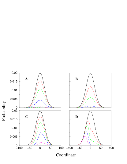
Figure 4: Probability density $p(x,t)$ at five times for two forces and diffusion coefficients: $D=10^{-10}$ and $10^{-15}$ cm${}^{2}/$s for the first and second row, and $f=10$ and 25 pN for the first and second column, respectively. The times are: 0, 175, 937, 1090, and 2700 ms. The distribution at 2700 ms in the panel B are too small to be showed.

When the diffusion coefficient is small, the diffusion along $x$ is practically frozen. Hence $p(x,t)$ will decay more on the side that k(x) is larger. Because both $\Delta G^{\ddagger}$ and $\xi^{\ddagger}$ are piecewise functions with two segments, we easily estimate the force, $f_{\rm e}=k_{g}/k_{\xi}$, at which all decay rates are independent of the coordinate $x$. Because f=10 pN and 25 pN are respectively smaller and larger than $f_{\rm e}=12.3$ pN given the current parameters, for the smaller force, the $p(x,t)$ decays more on the left side, while for the larger force, $p(x,t)$ decays more on the right side. Fig. 4C and D indeed indicate this prediction. In contrast, if the diffusion coefficient is large, the dissociation is slow compared to process of the conformational diffusion. The thermal equilibrium distribution of the conformations should be maintained during the courses of the dissociation “reaction”. It is cleanly seen in Fig. 4A and B. Because the single-molecule forced dissociation experiments usually measure the bond survival probability, we calculate $Q(t)$ for the same two diffusion coefficients and five forces; see Fig. 5.

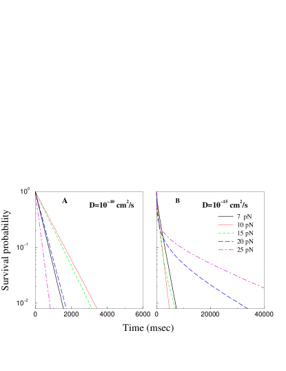
Figure 5: Survival probabilities vs. time at five forces for the two diffusion coefficients.

For the larger diffusion coefficient (Fig 5C), $Q(t)$s are almost monoexponential decays with time. We see that the decay first slows down with force increasing initially, and then speeds up when the force is beyond a threshold. These properties have been discussed in the rapid diffusion limit. More interesting case is from the smaller diffusion coefficients, e.g., $D=10^{-15}$ cm²s^-1 in Fig. 5D, where the main characteristics are completely different from the larger $D$ case. First, the survival probabilities exhibit highly stretched multiexponential decays. The trend becomes more apparent at larger forces. Second, the decay first speeds up and then slows down with force increasing. This abnormal behavior surprises us. It possibly means that the catch-slip bond transition in rapid diffusion limit converts into slip-catch transition when the diffusion is very slow along the conformational coordinate. In order to understand this behavior better, we consider the nondiffusion limit in which Eq. 3 has analytic solution.

III.3 nondiffusion limit: $D\to 0$

In this limit, according to Eq. 25, we get the mean lifetimes for the linear barrier and projection distance case (Eq. III.1),

$$\langle\tau\rangle(f) = k_{0}^{-1}\exp\left[\beta\Delta G^{\ddagger}_{0}+\frac{\beta}{2}\frac{k_{g}^{2}}{k_{x}}-\frac{\beta k_{x}}{2k^{2}_{\xi}}\left(\frac{k_{g}k_{\xi}}{k_{x}}+\xi^{\ddagger}_{0}\right)^{2}\right]$$ (46)

$$\times\exp\left[\frac{\beta k_{\xi}^{2}}{2k_{x}}\left(f-\frac{k_{g}k_{\xi}/k_{x}+\xi^{\ddagger}_{0}}{k_{\xi}^{2}/k_{x}}\right)^{2}\right],$$

and for the piecewise barrier and projection distance case,

$$\langle\tau\rangle(f) = \frac{k_{0}^{-1}}{2}\exp\left[\beta\Delta G_{0}^{\ddagger}+\frac{\beta}{2}\frac{k_{g}^{2}}{k_{x}}-\frac{\beta k_{x}}{2k^{2}_{\xi}}\left(\frac{k_{g}k_{\xi}}{k_{x}}+\xi^{\ddagger}_{0}\right)^{2}\right]$$

$$\times\exp\left[\frac{\beta k_{\xi}^{2}}{2k_{x}}\left(f-\frac{k_{g}k_{\xi}/k_{x}+\xi^{\ddagger}_{0}}{k_{\xi}^{2}/k_{x}}\right)^{2}\right]\times$$

$${\rm erfc}\left[-\sqrt{\frac{\beta k_{x}}{2}}\left(x_{b}-\frac{k_{g}}{k_{x}}+\frac{k_{\xi}}{k_{x}}f\right)\right]+$$

$$\frac{k_{0}^{-1}}{2}\exp\left[\beta\Delta G_{0}^{\ddagger}-\beta f\xi_{b}^{\ddagger}\right]{\rm erfc}\left[\sqrt{\frac{\beta k_{x}}{2}}x_{b}\right],$$

respectively. We see that, when force is larger enough, $k_{\xi}>0$ required in $D\to\infty$ case leads the mean lifetime of the piecewise case in the nondiffusion limit to increase rapidly in an exponential way of $f^{2}$. It proves our estimation. In addition, for the case of the linear barrier and projection distance, this catch behavior at larger forces even does not depend on any parameters. Fig. 6 shows how the mean lifetime of the PSGL-1$-$P-selectin bond changes with the decrease of $D$,

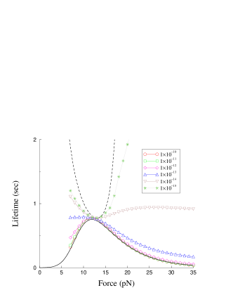
Figure 6: Mean lifetimes of the PSGL-1$-$P-selectin bond for six diffusion coefficients. The solid and dashed curves are respectively calculated by Eqs. III.1 and III.3 in $D\to\infty$ and $D\to$0 limits.

where same parameters are used. Compared to the counterintuitive catch-slip bond transitions, the slip-catch transitions presented here is physically inconceivable.

IV conclusions

Stimulated by the discovery of the catch-slip bond transitions in some biological adhesive bonds, several theoretical models have been developed to account for the intriguing phenomenon. According to the difference of the physical pictures, they can be divided into two classes. The first class is based on discrete chemical reaction schemes. They all assumed that there were two pathways and two or one energy well Evans2004 ; Barsegov ; Pereverzev . The applied force alters the fractions of the two pathways. The other class is based continuum diffusion-reaction models and mainly proposed by us liuf1 ; liuf2 . We cannot definitely distinguish which theory or model is the most reasonable and more close real situations, because their theoretical calculations all agree with the existing experimental data. In our opinion, the continuum models may be more attractive. In addition that the chemical kinetic models are clearly oversimplified, the most important cause is that the continuum models include an additional parameter, the diffusion coefficient $D$ liuf2 . The presence of the coefficient obliges the continuum diffusion-reaction models to face a strict test: it must be physically reasonable in the whole range of $D$. One of examples is that the present Bell rate model with dynamic disorder may be physically unacceptable because it predicts a slip-catch transition when the coefficient tends to zero. We have pointed our that the discrete chemical schemes may a mathematical approximation of the continuum model liuf2 . It is easy to see that the two pathway and one energy well model with a minus projection distance Pereverzev just corresponds the present model in the rapid diffusion limit. Therefore it is very possible that this chemical kinetic model also has a similar flaw. In contrast, FMDD model passes this test liuf2 . Of course, future experiments will finally decide which model is correct.

This work was supported in part by the National Science Foundation of China and the National Science Foundation under Grant No. PHY99-07949.

References

- (1) Bell, G. I. Science 1978, 200, 618.
- (2) Evans, E. and Ritchie, K. Biophys. J. 1997, 72, 1541.
- (3) Alon, R., Hammer, D. A., and Springer, T. A. Nature 1995, 374, 539.
- (4) Chen, S. and Springer, T. A. Proc. Natl. Acad. Sci. USA 2003, 98, 950.
- (5) Zwanzig, R. Acc. Chem. Res. 1990, 23, 148.
- (6) Wilemski, G. and Fixman, M. J. Chem. Phys. 1974, 60, 878.
- (7) Agmon, N. and Hopfield, J. J. J. Chem. Phys. 1983, 78, 6947.
- (8) Sumi, H. and Marcus, R. A. J. Chem. Phys. 1985, 84, 4894.
- (9) Bagchi, B., Fleming, G. R., and Oxtoby, D. W. J. Chem. Phys. 1983, 78, 7375.
- (10) Liu, F., Ou-Yang, Z.-C., and Iwamoto, M. Phys. Rev. E 2006, 73, 010901(R).
- (11) Liu, F. and Ou-Yang, Z.-C. q-bio.CB/0601017, submitted.
- (12) Marshall, B. T. et al. Nature 2003, 423, 190.
- (13) Dembo, M., Tourney, D. C., Saxman, K., and Hammer, D. Proc. R. Soc. Lond. B 1988, 234, 55.
- (14) Somers, W. S., Tang, J., Shaw, G. D., and Camphausen, R. T. Cell 2000, 103, 467.
- (15) McEver, R. P. Curr. Opin. Cell Biol. 2002, 14, 581.
- (16) Evans, E., Leung, A., Heinrich, V. and Zhu, C. Proc. Natl. Acad. Sci. USA 2004, 101, 11281.
- (17) Sarangapani, K. K. et al. J. Biol. Chem. 2003, 279, 2291.
- (18) Messiah, A. Quantum mechanics. North-Holland Pub. Co. Amsterdam, 1962.
- (19) Krissinel, E. B. and Agmon, N. J. 1996, 17, 1085.
- (20) Pereverzev, Y. V. et al. Biophys. J. 2005, 89, 1446.
- (21) Barsegov, V. and Thirumalai, D. Proc. Natl. Acad. Sci. USA 2005, 102, 1835.