Entanglement between static and flying qubits
in an Aharonov-Bohm double electrometer

Abstract

We consider the phase-coherent transport of electrons passing through an Aharonov-Bohm ring while interacting with a tunnel charge in a double quantum dot (representing a charge qubit) which couples symmetrically to both arms of the ring. For Aharonov-Bohm flux $\Phi_{\rm AB}=h/2e$ we find that electrons can only be transmitted when they flip the charge qubit’s pseudospin parity an odd number of times. The perfect correlations of the dynamics of the pseudospin and individual electronic transmission and reflection events can be used to entangle the charge qubit with an individual passing electron.

I Introduction

A scalable solid-state quantum computer has to rely on a hybrid architecture which combines static and flying qubits nielsen . Recent works propose the passage of electrons through mesoscopic scatterers for the generation of entanglement between flying qubits loss2000 ; burkard2000 ; Costa2001 ; Oliver2002 ; bose2002 ; Saraga2003 ; beenakkervelsen ; buettikersamuelsson ; Hu2004 , and charge measurements by an electrometer pepper have been proposed and realized to entangle or manipulate static spin and charge qubits dqdelectrometers ; ruskov ; emary ; engelloss ; trauzettel . Hence, it seems natural to exploit mesoscopic interference and scattering to entangle flying qubits to static qubits jefferson .

In this paper we demonstrate that prompt and perfect entanglement of a flying and a static charge qubit can be realized when a double quantum dot occupied by a tunnel charge is electrostatically coupled to the symmetric arms of an Aharonov-Bohm interferometer [an Aharonov-Bohm double electrometer, see Fig. 1(b)]. For an Aharonov-Bohm flux $\Phi_{\rm AB}=h/2e$ (half a flux quantum), each electron passing through the ring signals that the tunnel charge has changed its quantum state, while each electron which is reflected signals that the tunnel charge has maintained its state. This can be used to produce perfect entanglement between the static charge qubit represented by the tunnel charge in the double dot chargequbit , and the flying qubit represented by the charge of the conduction electron in the exit leads loss2000 ; burkard2000 ; Costa2001 ; Oliver2002 ; bose2002 ; Saraga2003 ; beenakkervelsen ; buettikersamuelsson ; Hu2004 . Since this entanglement mechanism does not require any energy fine tuning (for the implications of energy constraints see Ref. Hu2004 ), the entanglement can be produced quickly by the passage of a single electronic wave packet through the system.

Our proposal draws from both mesoscopic effects mentioned above — in essence, it consists of two electrometers both coupling to the same charge qubit, and pinched together to form an Aharonov-Bohm ring, which then represents a mesoscopic scatterer. Since we require that the coupling of the tunnel charge to the arms of the ring is symmetric, our proposal falls into the class of parity meters which have been discussed for the entanglement and detection of spin qubits emary ; engelloss and charge qubits trauzettel . In the present paper we are concerned with charge degrees of freedom only, and the resulting entanglement should be detectable by current-charge cross-correlation experiments beenakkervelsen ; buettikersamuelsson .

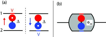
Figure 1: (Color online) Left panel: Schematic description of the double quantum dot (pseudospin $\uparrow$, $\downarrow$ depending on the occupation of the quantum dots, tunnel splitting $\Delta$), symmetrically coupled (via the potential $V$) to two quantum wires. Right panel: The Aharonov-Bohm double electrometer which results when the quantum wires are pinched together into an Aharonov-Bohm ring which is pierced by a magnetic flux $\Phi_{\rm AB}$.

II Scattering theory

In order to describe the properties of the Aharonov-Bohm double electrometer we start with the scattering region which is depicted in Fig. 1(a). It consists of two quantum wire segments labelled 1 and 2, which are symmetrically arranged around the double quantum dot. The tunnel charge in the double dot is described by a pseudospin, associated to states $|\uparrow\rangle$ when the charge is in the upper dot and $|\downarrow\rangle$ when the charge is in the lower dot. The ground state is given by the symmetric combination $|+\rangle=2^{-1/2}(|\uparrow\rangle+|\downarrow\rangle)$, and the excited state is $|-\rangle=2^{-1/2}(|\uparrow\rangle-|\downarrow\rangle)$. Both states are separated by a tunnel splitting energy $\Delta$. The orbital degree of freedom of the passing electron is described by basis states $|1\rangle$ and $|2\rangle$. Via its electrostatic repulsion potential $V(x)$, the tunnel charge impedes the current in wire $1$ when it occupies the upper dot, while it impedes the current in wire $2$ when it occupies the lower dot.

Outside of the range of the potential $V(x)$ one finds plane-wave scattering states

$$\psi_{s}=\sum_{\tau,\sigma,\eta=\pm}\psi_{\tau,s}(\eta k_{\sigma})\frac{\exp(i\eta k_{\sigma}x)}{\sqrt{2k_{\sigma}}}(|1\rangle+\tau|2\rangle)\otimes|\sigma\rangle,$$ (1)

where $k_{\sigma}=\frac{1}{\hbar}\sqrt{2m(E+\sigma\Delta)}$ for states of total energy $E$. The symbol $\eta=\pm$ describes the propagation direction along the wire, $\tau=\pm$ describes the orbital parity of the passing electron with respect to the wire segments $1$ and $2$, and $\sigma=\pm$ describes the pseudospin parity of the state of the double dot. For general scattering potential $V(x)$, the incoming and outgoing components are then related by an extended scattering matrix eplnoat

$$\widetilde{S}=\left(\begin{array}[]{cccc}\tilde{r}_{++}&\tilde{r}_{+-}&\tilde{t}^{\prime}_{++}&\tilde{t}^{\prime}_{+-}\\ \tilde{r}_{-+}&\tilde{r}_{--}&\tilde{t}^{\prime}_{-+}&\tilde{t}^{\prime}_{--}\\ \tilde{t}_{++}&\tilde{t}_{+-}&\tilde{r}^{\prime}_{++}&\tilde{r}^{\prime}_{+-}\\ \tilde{t}_{-+}&\tilde{t}_{--}&\tilde{r}^{\prime}_{-+}&\tilde{r}^{\prime}_{--}\\ \end{array}\right),$$ (2)

which takes the initial and final state of the tunnelling charge into account:

$$\left(\begin{array}[]{c}\psi_{+,l}(-k_{+})\\ \psi_{-,l}(-k_{-})\\ \psi_{+,r}(k_{+})\\ \psi_{-,r}(k_{-})\\ \end{array}\right)=\widetilde{S}\left(\begin{array}[]{c}\psi_{+,l}(k_{+})\\ \psi_{-,l}(k_{-})\\ \psi_{+,r}(-k_{+})\\ \psi_{-,r}(-k_{-})\\ \end{array}\right),$$ (3)

$$\left(\begin{array}[]{c}\psi_{-,l}(-k_{+})\\ \psi_{+,l}(-k_{-})\\ \psi_{-,r}(k_{+})\\ \psi_{+,r}(k_{-})\\ \end{array}\right)=\widetilde{S}\left(\begin{array}[]{c}\psi_{-,l}(k_{+})\\ \psi_{+,l}(k_{-})\\ \psi_{-,r}(-k_{+})\\ \psi_{+,r}(-k_{-})\\ \end{array}\right).$$ (4)

Analogously, the complete Aharonov-Bohm double electrometer in Fig. 1(b) is described by an extended scattering matrix

$$S=\left(\begin{array}[]{cccc}r_{++}&r_{+-}&t^{\prime}_{++}&t^{\prime}_{+-}\\ r_{-+}&r_{--}&t^{\prime}_{-+}&t^{\prime}_{--}\\ t_{++}&t_{+-}&r^{\prime}_{++}&r^{\prime}_{+-}\\ t_{-+}&t_{--}&r^{\prime}_{-+}&r^{\prime}_{--}\\ \end{array}\right).$$ (5)

The amplitudes $r_{\pm,\pm}$ ($r^{\prime}_{\pm,\pm}$) are associated to reflection from the left (right) lead, and the amplitudes $t_{\pm,\pm}$ ($t^{\prime}_{\pm,\pm}$) are associated to transmission from left to right (right to left), while the first (second) subscript denotes the state of the tunnelling charge after (before) the passage of the electron through the ring.

The matrix $S$ can be related to the internal scattering matrix $\tilde{S}$ by adopting the standard model for an Aharonov-Bohm ring developed in Ref. imry . The contacts to the left ($s=L$) and right ($s=R$) lead are characterized by reflection amplitudes $\alpha_{s}$ and transmission amplitudes $\beta_{s}=\sqrt{1-\alpha_{s}^{2}}$ which describe the coupling into the symmetric orbital parity state $2^{-1/2}(|1\rangle+|2\rangle)$. The Aharonov-Bohm flux $\Phi_{\rm AB}$ mixes the symmetric and antisymmetric orbital parities in the passage from one contact to the other contact by a mixing angle $\phi=\pi\Phi_{\rm AB}e/h$. The lengths of the ballistic regions between the scattering region and the left and right contact are denoted by $d_{L}$ and $d_{R}$, respectively.

The total scattering matrix is then of the form

$$S=-\alpha+\beta(A^{\dagger}-\alpha-B^{\dagger}[A^{\dagger}+1]^{-1}B^{\dagger})^{-1}\beta,$$

$$A=\gamma\left(\begin{array}[]{cccc}\tilde{r}_{++}&0&c\tilde{t}^{\prime}_{++}&-is\tilde{t}^{\prime}_{+-}\\ 0&\tilde{r}_{--}&-is\tilde{t}^{\prime}_{-+}&c\tilde{t}^{\prime}_{--}\\ c\tilde{t}_{++}&is\tilde{t}_{+-}&\tilde{r}^{\prime}_{++}&0\\ is\tilde{t}_{-+}&c\tilde{t}_{--}&0&\tilde{r}^{\prime}_{--}\\ \end{array}\right)\gamma,$$ (10)

$$B=\gamma\left(\begin{array}[]{cccc}0&\tilde{r}_{+-}&-is\tilde{t}^{\prime}_{++}&c\tilde{t}^{\prime}_{+-}\\ \tilde{r}_{-+}&0&c\tilde{t}^{\prime}_{-+}&-is\tilde{t}^{\prime}_{--}\\ is\tilde{t}_{++}&c\tilde{t}_{+-}&0&\tilde{r}^{\prime}_{+-}\\ c\tilde{t}_{-+}&is\tilde{t}_{--}&\tilde{r}^{\prime}_{-+}&0\\ \end{array}\right)\gamma,$$ (15)

$\alpha={\rm diag}(\alpha_{L},\alpha_{L},\alpha_{R},\alpha_{R})$, $\beta={\rm diag}(\beta_{L},\beta_{L},\beta_{R},\beta_{R})$, $\gamma={\rm diag}\,(e^{ik_{+}d_{L}},e^{ik_{-}d_{L}},e^{ik_{+}d_{R}},e^{ik_{-}d_{R}})$, $c=\cos\phi$, $s=\sin\phi$.

III Degree of entanglement

III.1 Stationary concurrence

The scattering amplitudes of the extended scattering matrix (5) can now be used to assess how the tunnel charge on the double dot becomes entangled with the itinerant electron during its passage through the Aharonov-Bohm double electrometer. In particular, they describe by which lead the passing electron exits and how this is correlated to the final state of the double dot. We assume that the double dot is initially in the symmetric state $|+\rangle$ and hence uncorrelated to an arriving electron that enters the ring from the left lead. The degree of entanglement between the final state of the double dot and the exit lead of the electron can then be quantified by the concurrence concurrence

$${\cal C}=2|r_{++}t_{-+}-r_{-+}t_{++}|,$$ (16)

which provides a monotonous measure of entanglement (${\cal C}=0$ for unentangled states and ${\cal C}=1$ for maximal entanglement).

For the case of a vanishing flux $\Phi_{\rm AB}=0$, the mixing angle is $\phi=0$. It then follows from Eq. (15) that the scattering matrix is of the form

$$S=\left(\begin{array}[]{cccc}r_{++}&0&t^{\prime}_{++}&0\\ 0&r_{--}&0&t^{\prime}_{--}\\ t_{++}&0&r^{\prime}_{++}&0\\ 0&t_{--}&0&r^{\prime}_{--}\\ \end{array}\right).$$ (17)

In this case the electron can only leave the system when the pseudospin of the scatterer has flipped an even number of times, hence the final state of the scatterer is identical to its initial state. There is no entanglement, and consequently the concurrence (16) vanishes, ${\cal C}=0$.

For $\Phi_{\rm AB}=h/2e$, the mixing angle is $\phi=\pi/2$, and the scattering matrix is of the form

$$S=\left(\begin{array}[]{cccc}r_{++}&0&0&t^{\prime}_{+-}\\ 0&r_{--}&t^{\prime}_{-+}&0\\ 0&t_{+-}&r^{\prime}_{++}&0\\ t_{-+}&0&0&r^{\prime}_{--}\\ \end{array}\right).$$ (18)

Now the electron becomes entangled with the double dot: the electron is reflected when the double dot is finally in its symmetric state (the pseudospin of the double dot has then flipped an even number of times), while the electron is transmitted when the double dot is finally in its antisymmetric state (it then has flipped an odd number of times). The concurrence ${\cal C}=2|r_{++}t_{-+}|$ signals perfect entanglement, ${\cal C}=1$, when the probabilities of reflection and transmission are identical, $|r_{++}|^{2}=|t_{-+}|^{2}=1/2$. The condition for perfect entanglement corresponds to the case of maximal shot noise beenakkervelsen ; buettikersamuelsson .

The entanglement in the Aharonov-Bohm double electrometer results because the total parity $\sigma\tau$ is conserved in the scattering from the double quantum dot. This conservation law yields the separate Eqs. (3,4), which only couple wave components of the same total parity. Since the scattering matrix $\widetilde{S}$ for positive and negative total parity is identical, this realizes a parity meter which entangles the orbital parity of the passing electron to the pseudospin parity of the double dot. The role of the Aharonov-Bohm ring with flux $\Phi=h/2e$ is to convert the orbital parity into charge separation in the exit leads. When the electron enters the ring at the left contact, this prepares it locally in the orbitally symmetric state. Neglecting the scattering from the double dot, the electron cannot leave at the right contact since it will end up there in the antisymmetric orbital state. Transmission is therefore only possible if the orbital parity is flipped by interaction with the tunnel charge. But since the total parity is preserved, this scattering event is necessarily accompanied by a parity change of the double dot. Consequently, the final state of the tunnel charge is perfectly correlated to the lead by which the passing electron leaves the Aharonov-Bohm double electrometer.

III.2 Time-dependent concurrence

The energy-dependent scattering matrix (5) and the expression (16) for the concurrence describe the stationary transport through the system. A pressing issue for many proposals involving flying qubits is that they require an energy fine tuning which entails a degrading of the entanglement in the time domain Hu2004 . As we will now show, the entanglement can in fact be increased above the value of the stationary concurrence when a single electronic wave packet is passed through the Aharonov-Bohm electrometer with $\Phi_{\rm AB}=h/2e$.

In this non-stationary situation, the entanglement is quantified by the time-dependent concurrence

$${\cal C}(t)=2\Big{|}\langle\psi_{+}|\psi_{+}\rangle\langle\psi_{-}|\psi_{-}\rangle-|\langle\psi_{+}|\psi_{-}\rangle|^{2}\Big{|}^{1/2},$$ (19)

where $\psi_{+}$ and $\psi_{-}$ are the orbital wavefunctions obtained by projection onto the symmetric and antisymmetric state of the double dot, respectively. The potential for entanglement enhancement follows from the lower bound

$${\cal C}(t)>{\cal C}_{\rm min}(t)=2\sqrt{P_{L}(t)P_{R}(t)-\frac{1}{4}P_{0}(t)^{2}}$$ (20)

of the time-dependent concurrence, which can be derived directly from the form (18) of the scattering matrix when one assumes that the wave packet has completely entered the ring. Here $P_{L}(t)$ is the weight of the reflected wave packet, $P_{R}(t)$ is the weight of the transmitted wave packet, and $P_{0}(t)=1-P_{L}(t)-P_{R}(t)$ is the weight of the wave packet in the ring. For large times $P_{0}(t=\infty)=0$, and the weights $P_{L}(t=\infty)=R$ and $P_{R}(t=\infty)=T$ give the reflection and transmission probabilities of the wave packet, which can be obtained by an energy average over the wave packet components. For the case that this energy average yields equal reflection and transmission probabilities $R=T=1/2$, the final value of the concurrence after passage of the electron is $C(t=\infty)=1$. In this case, maximal entanglement results during the passage of the electron through the system – independent of the precise dependence of the stationary concurrence in the energetic range of the wave packet. This entanglement enhancement is only possible because the scattering matrix $S$ retains its sparse structure (18) for all energies.

To give a specific example, we consider the case that the tunnelling charge induces a localized scattering potential $V=\frac{\hbar^{2}}{2m}g\delta(x)$ in the quantum wire. This problem can be solved exactly for arbitrary values of the tunnel splitting $\Delta$, scattering strength $g$, and ring parameters $d_{s}$ and $\alpha_{s}$, using the technique of Ref. eplnoat . Here we concentrate on the case of a vanishing tunnel splitting $\Delta=0$, strong scattering $g\to\infty$, transparent contacts with $\alpha_{R}=\alpha_{L}=0$, and equal distance $d_{L}=d_{R}\equiv d$ of the double dot to the contacts. The extended scattering matrix is then of the form

$$S=-e^{3ikd}\left(\begin{array}[]{cccc}\tilde{c}&0&i\tilde{s}c&-\tilde{s}s\\ 0&\tilde{c}&-\tilde{s}s&i\tilde{s}c\\ i\tilde{s}c&\tilde{s}s&\tilde{c}&0\\ \tilde{s}s&i\tilde{s}c&0&\tilde{c}\\ \end{array}\right),$$ (21)

where $\tilde{c}=\cos kd$ and $\tilde{s}=\sin kd$.

At fixed energy, the stationary concurrence (16) is given by ${\cal C}=|\sin\phi\sin 2kd|$, and the maximal stationary concurrence ${\cal C}=|\sin 2kd|$ is attained at $\phi=\pi/2$, corresponding to $\Phi_{\rm AB}=h/2e$. The factor $|\sin 2kd|$ arises from the energy dependence of the reflection probability $R=\cos^{2}kd$. For a narrow wave packet, the reflection and transmission probabilities average to $1/2$, and the time-dependent concurrence approaches the maximal value ${\cal C}(t=\infty)=1$ for large times.

In order to assess the time scale on which the entangled state is formed we have performed numerical simulations which are presented in Fig. 2. The wave packet was propagated by a second-order Crank-Nicholson scheme, and the Aharonov-Bohm ring and the leads were formed by tight-binding chains at wavelengths much larger than the lattice constant. For a narrow wave packet, the simulations confirm that the final state is perfectly entangled. For broader wave packets, the final entanglement is not necessarily perfect and depends on the average wave number, but is always attained on a time scale comparable to the propagation time of the wave packet between the contacts in the ring.

In Fig. 3 we assess how the degree of entanglement for a narrow wave packet depends on the scattering strength $g$. Perfect entanglement is obtained for $g\gtrsim 0.1$, hence, already for rather weak coupling. For smaller $g$, the entanglement produced by a single passage of the wave packet is reduced. As required, the entanglement vanishes altogether in the limit $g\to 0$. For small but finite $g$, one should expect that the entanglement can be enhanced by multiple passage of the wave packet through the ring, which can be achieved by isolating the system for a finite duration from the external electrodes (e.g., by pinching off the external wires via the voltage on some split gates). This expectation is confirmed in Fig. 4, which shows the time-dependent concurrence for a narrow wave packet which passes through the ring and is reflected at hard-wall boundaries in the external wires, at a distance of $4000\,a$ to either side of the ring.

Figure 2: Time-dependent concurrence when an electronic wave packet passes through the ring with Aharonov-Bohm flux $\Phi_{AB}=h/2e$, while the double quantum dot is initially in its symmetric state. The scattering potential is $V=\frac{\hbar^{2}}{2m}g\delta(x)$ with $g\to\infty$. The contacts to the ring are transparent, $\alpha_{R}=\alpha_{L}=0$. The distance $d_{L}=d_{R}\equiv d$ of the double dot to the contacts is $d=125\,a$ , where $a$ is the lattice constant. Time is measured in units of the average time of flight $t_{D}=2d/\langle v\rangle$ of the wave packet between the two contacts. The center of the initial wave packet in the lead is at a distance of $2000\,a$ to the ring. The initial widths $w$ and the average wave numbers $\langle k\rangle$ are: $w=0.2d$, $\langle k\rangle d=4\pi$ (solid curve), $w=2d$, $\langle k\rangle d=4\pi$ (dashed curve), $w=2d$, $\langle k\rangle d=4.125\pi$ (dotted curve), $w=2d$, $\langle k\rangle d=4.25\pi$ (dashed-dotted curve).

Figure 3: Time-dependent concurrence for the narrow wave packet with $w=0.2d$ and $\langle k\rangle d=4\pi$ described in Fig. 2, but now calculated for finite values of the coupling strength $g=0.001$, $0.002$, $0.003$, $0.004$, $0.005$, $0.01$, $0.1$ (bottom to top).

Figure 4: Solid line: Time-dependent concurrence for the narrow wave packet with $w=0.2d$ and $\langle k\rangle d=4\pi$ described in Fig. 2, but for $g=0.001$ and a set-up in which the wires are terminated by hard walls at a distance $4000\,a$ to either side of the ring. The concurrence is enhanced due to the multiple passages of the wave packet through the ring. The dashed line shows the probability $P_{0}(t)$ of the propagating electron to reside in the ring, which is revived in the multiple passages through the ring.

III.3 Sensitivity to decoherence and asymmetries

The time-dependent scattering analysis of the entanglement mechanism reveals an important and rather unique feature of the proposed device: As the entanglement can be generated in a single quasi-instantaneous scattering event, the proposed mechanism is rather robust against decoherence from time-dependent fluctuations of the environment (decoherence, however, will always become important in the subsequent dynamics of the system nielsen ). The main source of entanglement degradation hence comes from imperfections in the fabrication of the device itself, and here especially from imperfections which break the parity symmetry of the set-up. Arguably the most critical part of the set-up is the requirement of symmetric coupling to the double dot, as other asymmetries (in the arm length and contacts to the external wires) are just of the same character as in the conventional Aharanov-Bohm effect and can be partially compensated, e.g., via off-setting the magnetic flux. The sensitivity to asymmetries in this coupling is explored in Fig. 5, where the coupling strength to one arm is fixed to $g=0.1$ while in the arm the strength is reduced by a factor $\alpha$. Astonishingly, a rather large degree of entanglement remains even for much reduced $\alpha$, which indicates that the proposed mechanism is rather more robust to asymmetries than it could have been expected.

Figure 5: Time-dependent concurrence for the narrow wave packet with $w=0.2d$ and $\langle k\rangle d=4\pi$ described in Fig. 2, but for asymmetric coupling to the double dot. In one arm, the coupling strength is $g=0.1$ while in the other arm it is reduced by a factor $\alpha=1$, $0.1$, $0.05$, and $0$ (top to bottom).

IV Discussion and conclusions

In conclusion, we have demonstrated that a tunnel charge on a double quantum dot can be entangled to an individual electron which passes through an Aharonov-Bohm ring with flux $\Phi_{\rm AB}=h/2e$. Ideal operation requires symmetric electrostatic coupling of the tunnel charge to the two arms of the ring. The entangled state is produced quickly, on time scales comparable to the passage of the electron through the ring. Since the entanglement in principle is generated in a single quasi-instantaneous scattering event, the proposed mechanism is robust against decoherence.

The mesoscopic components for the proposed entanglement circuit – double quantum dots, ring geometries of quantum wires, and charge electrometers based on the electrostatic coupling of quantum dots to quantum wires – have been realized and combined in numerous experiments over the past decade, and recently the dynamics of static qubits in double quantum dots has been monitored successfully chargequbit ; dqdelectrometers . An initial experiment would target the finite conductance of the mesoscopic ring at half a flux quantum, $\Phi_{\rm AB}=h/2e$, where the conventional Aharonov-Bohm effect would yield total destructive interference and hence no current. The shot noise provides an indirect measurement of the underlying correlated dynamics of the tunnel charge and the mobile electron. A direct experimental investigation of the ensuing entanglement requires to measure the correlations between the individual transmission and reflection events and the pseudospin dynamics of the double quantum dot. The cross-correlation measurements could be carried out with a stationary stream of electrons, at a small bias $V<t_{D}/e\hbar$ (hence an attempt frequency less than the typical dwell time $t_{D}$ of an electron in the ring). As in other proposals involving flying qubits, the incoming stream of electrons can be further diluted by a tunnel barrier in the lead from the electronic source. In a more sophisticated setting, a single charge would be driven into the system via an electronic turnstile turnstile . It also may be desirable to lead the reflected or transmitted charges into dedicated channels via electronic beam splitters or chiral edge states Ji .

We thank C. W. J. Beenakker and T. Brandes for helpful discussions. This work was supported by the European Commission, Marie Curie Excellence Grant MEXT-CT-2005-023778 (Nanoelectrophotonics).

References

- (1) M. L. Nielsen and I. L. Chuang, Quantum Computation and Quantum Information (Cambridge University Press, Cambridge, 2000).
- (2) D. Loss and E. V. Sukhorukov, Phys. Rev. Lett. 84, 1035 (2000).
- (3) G. Burkard, D. Loss, and E. V. Sukhorukov, Phys. Rev. B. 61, R16303 (2000).
- (4) A. T. Costa, Jr. and S. Bose, Phys. Rev. Lett. 87, 277901 (2001).
- (5) W. D. Oliver, F. Yamaguchi, and Y. Yamamoto, Phys. Rev. Lett. 88, 037901 (2002).
- (6) D. S. Saraga and D. Loss, Phys. Rev. Lett. 90, 166803 (2003).
- (7) C. W. J. Beenakker, C. Emary, M. Kindermann, and J. L. van Velsen, Phys. Rev. Lett. 91, 147901 (2003).
- (8) P. Samuelsson, E. V. Sukhorukov, and M. Büttiker, Phys. Rev. Lett. 92, 026805 (2004).
- (9) S. Bose and D. Home, Phys. Rev. Lett. 88, 050401 (2002).
- (10) X. Hu and S. Das Sarma, Phys. Rev. B 69, 115312 (2004).
- (11) M. Field et al., Phys. Rev. Lett. 70, 1311 (1993); E. Buks et al., Nature 391, 871 (1998).
- (12) R. Ruskov and A. N. Korotkov, Phys. Rev. B 67, 241305(R) (2003).
- (13) C. W. J. Beenakker, D. P. DiVincenzo, C. Emary, and M. Kindermann, Phys. Rev. Lett. 93, 020501 (2004).
- (14) H.-A. Engel and D. Loss, Science 309, 586 (2005).
- (15) B. Trauzettel, A. N. Jordan, C. W. J. Beenakker, and M. Büttiker, Phys. Rev. B 73, 235331 (2006).
- (16) J. M. Elzerman et al., Nature (London) 430, 431 (2004); J. R. Petta et al., Phys. Rev. Lett. 93, 186802 (2004); Science 309, 2180 (2005); F. H. L. Koppens et al., Science 309, 1346 (2005).
- (17) J. H. Jefferson, A. Ramšak, and T. Rejec, Europhys. Lett. 74, 764 (2006); D. Gunlycke, J. H. Jefferson, T. Rejec, A. Ramšak, D. G. Pettifor, and G. A. D. Briggs, cond-mat/0511126 (2005).
- (18) T. Hayashi, T. Fujisawa, H. D. Cheong, Y. H. Jeong, and Y. Hirayama, Phys. Rev. Lett. 91, 226804 (2003); J. Gorman, E. G. Emiroglu, D. G. Hasko, and D. A. Williams, Phys. Rev. Lett. 95, 090502 (2005).
- (19) H. Schomerus, Y. Noat, J. Dalibard, and C. W. J. Beenakker, Europhys. Lett. 57, 651 (2002).
- (20) M. Büttiker, Y. Imry, and M. Ya. Azbel, Phys. Rev. A 30, 1982 (1984).
- (21) W. K. Wootters, Phys. Rev. Lett. 80, 2245 (1998).
- (22) L. P. Kouwenhoven et al., Phys. Rev. Lett. 67, 1626 (1991).
- (23) Y. Ji, Y. Chung, D. Sprinzak, M. Heiblum, D. Mahalu, and H. Shtrikman, Nature (London) 422, 415 (2003).