Duality and phase diagram of one dimensional transport

Abstract

The observation of duality by Mukherji and Mishra in one dimensional transport problems has been used to develop a general approach to classify and characterize the steady state phase diagrams. The phase diagrams are determined by the zeros of a set of coarse-grained functions without the need of detailed knowledge of microscopic dynamics. In the process, a new class of nonequilibrium multicritical points has been identified.

1 Introduction

There are many situations that involve transport of particles from one end to other along a one dimensional track obeying some form of mutual exclusion[1]. Examples are vehicular traffic in a one-lane road, molecular motors carrying cargo on a track in biological systems and so on. Moreover, such simple systems are of importance to develop an understanding of nonequilibrium steady state phases and phase transitions.

Many such transport models have now been studied extensively via analytical methods, meanfield approximations and numerical simulations, and different types of phases have been identified[2, 3, 4, 5, 6, 7, 8]. These phases are represented in phase diagrams in the space of the externally controllable parameters of the problem, namely, the imposed rates of injection and withdrawal at the two boundaries. The fact that the boundary conditions determine the stable phase diagrams makes these nonequilibrium problems different from equilibrium ones.

Since phase transitions involve the whole of the system, the generic behavior, in the large size limit, is expected to be determined by certain gross overall features. This is the way equilibrium phase transitions are analyzed, but, alas, no such general framework is known for nonequilibrium cases. Hence the efforts on case by case studies. Our aim is to develop a general formulation at least for the above class of systems. We show that the generic features and the universal properties of the phase diagrams can be obtained from the structure of a set of $S$-functions and by using a recently discovered duality[3], without the need of detailed specifics of the microscopic dynamic rules and interaction. Still, one microscopic parameter remains essential for the problem, namely, a small distance cutoff (e.g. lattice spacing or some microscopic size etc) which cannot blindly be set to zero. The usefulness of the approach is shown by predicting a new class of nonequilibrium multicritical points.

2 Phases and response functions

As an example[2, 3, 8], consider a one dimensional lattice of $N(\to\infty)$ sites. Particles are injected at site $i=1$ at a rate $\alpha$ (i.e probability that a particle is injected in a short time interval $dt$ is $\alpha dt$) and withdrawn at site $i=N$ at a rate $1-\gamma$. The particles hop on the lattice as per preassigned rules, like forbidden multiple occupancy of a site, etc. In addition, non-conserving processes may allow addition to or deletion from the track at rates $\omega_{a}$ and $\omega_{d}$ respectively, as e.g., exits or feeders in a traffic system for cars to get out of or into the road, or “processive”objects in biological systems falling off the track or getting reattached from the bulk solution. The parameters, $K=\omega_{a}/\omega_{d}$ and $\Omega=\omega_{d}N$ are characteristics of the microscopic dynamics while $\alpha$ and $\gamma$ are externally imposed.

For a coarse-grained description, the natural variable is the local density or the space-time dependent average occupation number $\rho(x,t)$ in continuum ($x\in[0,1]$ by a rescaling of the total length). The sensitivity to the boundary concentrations (or rates) can be measured by the response functions

$$\chi_{\mu}\equiv\frac{\partial M}{\partial\mu},\ {\rm where}\ \mu=\alpha\ {\rm or}\ \gamma,{\rm and}\ M=\int_{0}^{1}\!\!dx\ \rho(x),$$ (1)

is the steady state spatially averaged density. Any two points in the $\alpha-\gamma$ space are said to be in the same phase if they can be connected by a continuous path along which the density profile or the response functions change smoothly. Any point of non-analyticity on a path defines the location of the phase transition.

The phases observed are, generally, of the following types. (i) Injection (withdrawal) rate dominated, to be called the $\alpha$-phase ($\gamma$-phase), (ii) a shock phase consisting of piecewise continuous densities, and (iii) special phases. In the shock phase, there is a discontinuity in the density separating an $\alpha$-phase on one side from a $\gamma$-phase on the other side, while an example of (iii) is a phase where the current through the system is maximum. The response functions behave differently in these phases. In the $\alpha$-phase, $\chi_{\alpha}\sim O(1)$ but $\chi_{\gamma}=0$, while in the $\gamma$-phase, it is the other way round. However, in the shock phase, both $\chi_{\alpha}$ and $\chi_{\gamma}$ would be nonzero. For special phases like (iv) in the above list, $\chi_{\alpha,\gamma}\approx 0$.

3 Equations for dynamics and steady states: Definitions of $S_{i}$’s

In a continuum limit for large $N$ (with lattice spacing $a\ll L=Na$) the time variation of $\rho(x,t)$ can be written in the form of a continuity equation, as

$$\frac{\partial\rho(x)}{\partial t}+\frac{\partial J_{0}(x,t)}{\partial x}=S_{0}(\rho,t),$$ (2)

where the right hand side is the explicit non-conserving contribution to the change in density. The left hand side is in the form of a continuity equation with $J_{0}(x,t)$ as the current at the site. In a mean field approximation, the current is taken to be an implicit function of position and time through the density, so that $J_{0}$ can be split into two parts,

$$J_{0}=-\epsilon S_{2}(\rho)\frac{\partial\rho}{\partial x}+J(\rho(x,t)),$$ (3)

with a “bulk” contribution $J(\rho)$ determined by the local density and a term that depends on the derivative of the density (“Fick’s law”) over the lattice spacing, $\epsilon=a/2N$ being small. This $\epsilon$-dependent term is a reminiscent of the interactions in the neighborhood of a site on the underlying lattice. The form of $S_{2}(\rho)$ is determined by the microscopic dynamics, but, for simplicity, we take $S_{2}(\rho)=1$ here. Such a form like Eq. 3 has recently been shown by Chakrabarti[9] to arise naturally in a renormalization group type approach for transport processes and failures of fiber bundles. The fact that there are two fixed points (viewed as a recursion relation) will be of importance to us also.

In the steady state, the system evolves to a time independent density profile satisfying

$$-\epsilon\frac{d\ }{dx}S_{2}(\rho)\frac{d\rho}{dx}+S_{1}(\rho)\frac{d\rho}{dx}+S_{0}(\rho)=0.$$ (4)

The $S_{i}$ functions encode the dynamics or specialties of the system. The density satisfies the boundary conditions $\rho(0)=\alpha$ and $\rho(1)=\gamma$. The microscopic rules are taken to be sufficiently smooth to warrant considerations of smooth and analytic functions only. These restrictions can be relaxed if necessary.

For $\epsilon\to 0$, the ensuing first order equation cannot in general satisfy the two boundary conditions. Therefore, the $\epsilon$ term, eventhough looks innocuous in the bulk limit, is essential. It defines a new scale ${\tilde{x}}=x/\epsilon$ in the problem and this scale is important for the phase transitions. E.g., the discontinuity at a shock will be rounded on a scale of ${\tilde{x}}$ but would look sharp on a bigger scale.

3.1 Nature of $S_{0}$

Let us first consider the role and the nature of $S_{0}(\rho)$. The zero of the non-conservation function $S_{0}(\rho)$ is a special density. This is the equilibrium like steady state density $\rho=\rho_{L}$, $S_{0}(\rho_{L})=0$, the system would evolve to if all other dynamics, except this non-conserving one, are switched off. In such a situation, the density $\rho_{L}$ can be obtained from the extrema of a (free energy like) Lyapunov function, ${\hat{S}}_{0}(\rho)$ such that $S_{0}(\rho)=-d{\hat{S}_{0}}/d\rho$. For stability of the state, evaporation is to be preferred in case of excess density (over $\rho_{L}$), but adsorption for $\rho<\rho_{L}$. This requires $S_{0}(\rho)$ to be an odd function or, ${\hat{S}}_{0}(\rho)$ an even function of $\rho-\rho_{L}$. A simple possible choice is

$${\hat{S}}_{0}(\rho)=\Omega(\rho-\rho_{L})^{2q},\ (q\geq 1),$$ (5)

with $q=1$ corresponding to a linear form for $S_{0}$ (the so-called Langmuir kinetics). The “softness”of the state is determined by the parameter $\Omega$ that controls the width of the well. Also, the conserved case is recovered by taking $\Omega\to 0$. A bistable (or multi-stable) situation can be obtained for $\Omega<0$ with additional terms in ${\hat{S}}_{0}$.

3.2 Nature of $S_{1}$

A zero of $S_{1}(\rho)$, i.e. $S_{1}(\rho_{m})=0$, is the density at which the current is an extrema (e.g. a maximum). From Eq. (4), we see that this is the density where one may afford a non-existence of the first derivative of the density. Consequently, a shock, for which the derivative is not defined (strictly in the $\epsilon\to 0$ limit), if exists, has to be centered around $\rho=\rho_{m}$. If the dynamics has a particle hole symmetry, then $\rho_{m}=1/2$. For concreteness and simplicity we consider the class of functions

$$J(\rho)\approx J_{\rm m}-a(\rho-\rho_{m})^{2p},\ (p\geq 1),$$ (6)

near the maximum. There can be cases with more than one zero of $S_{1}(\rho)$, which can lead to multiple shocks and more exotic phenomena. Such cases will be discussed elsewhere.

3.3 Special cases

The microscopic dynamic rules determine the values of the two special densities, $\rho_{L},\rho_{m}$, and the values of $p,q$. However, we do not require those rules. We need to distinguish special cases like, (i) $\rho_{L}>\rho_{m}$, (ii) $\rho_{L}<\rho_{m}$,and (iii) $\rho_{L}=\rho_{m}$. It is plausible to make a smoothness hypothesis that the nature of the phase diagram in the $\alpha-\gamma$ (external)-parameter space changes smoothly as the parameters like $\rho_{l},\rho_{m}$ (determined by the microscopics) are changed unless there is a special condition. Such a condition is $\rho_{L}=\rho_{m}$ where the non-conserving processes try to maintain a density at which the conserved processes can accommodate maximum current.

4 Boundary layer approach: outer and inner densities

We adopt the boundary layer approach or the method of matched asymptotics to handle the two scales in Eq. (4). Consider the case where the bulk density profile $\rho=\rho_{\rm out}(x)$, obtained from Eq. 4 with $\epsilon=0$, matches the boundary condition $\rho(x=0)$ = $\alpha$. But, then, $\rho_{\rm o}$ $\equiv\rho_{\rm out}(x=1)$ $\neq\gamma$. A different density profile $\rho_{\rm in}({\tilde{x}})$ where ${\tilde{x}}=(x-x_{s})/\epsilon$ $\sim O(1)$, $(x_{s}=1)$, extrapolates within a thin “inner” region from $\rho_{\rm in}(-\infty)=\rho_{\rm o}$ to $\rho_{\rm in}(0)=\gamma$. This inner region satisfies $\left({\rm see\ Eq.\ref{eq:5}},\ S_{1}(\rho)={d{\hat{S}}_{1}(\rho)}/{d\rho}\right)$

$$-S_{2}(\rho_{\rm in})\frac{d\rho_{\rm in}}{d{\tilde{x}}}+{\hat{S}}_{1}(\rho_{\rm in})=0,$$ (7)

which is equivalent to Eq. 3 with ${\hat{S}}_{1}(\rho)=J(\rho)-J_{0}$. The inner region, to first order in $\epsilon$, is too thin for the violation of conservation to matter, so that the current $J_{0}=J(\rho_{\rm o})$ entering from the bulk (outer) region remains conserved in the inner layer. Inference: The mandatory matching condition requires ${\hat{S}}_{1}(\rho)$ to have a zero at $\rho=\rho_{\rm o}$.

4.1 Zeros as requirements for shocks

A shock is formed only if the inner solution fails to satisfy the boundary condition. This happens if the inner solution saturates at the other end. Therefore the minimal requirement for shock formation is another zero of ${\hat{S}}_{1}(\rho)$, so that

$${\hat{S}}_{1}(\rho)=-(\rho-\rho_{\rm o})(\rho-\rho_{\rm s})\Phi(\rho).$$ (8)

The first nontrivial case, is therefore a function with two simple zeros and $\Phi(\rho)=1$. The two zeros $\rho_{\rm o}$ and $\rho_{s}$ correspond to the two fixed points of Chakrabarti’s approach[9]. By Rolle’s theorem, $\rho_{\rm o}\leq\rho_{m}\leq\rho_{\rm s}$.

The inner equation admits two types of solutions, one bounded (B-type) between $\rho_{o}$ and $\rho_{s}$ while the other one shows a divergence (U-type) with $d\rho/dx\sim-\rho^{2}$, or more generally, $d\rho/dx\sim-\rho^{2p}$. It is the B-type layers that matures to a shock but not the U-type. The inner solution is of the form ${\cal I}({\tilde{x}}/w+\xi)$ with ${\cal I}(z)\to\rho_{s}$ or $\rho_{\rm o}$ as $z\to\pm\infty$. Here $w$ is the width of the layer and $\xi$ gives the location of the center of the layer. So instead of the two boundary conditions describing the layer, we may instead opt for the $w,\xi$ pair. The center may lie outside the physical range or may be in an unphysical density range, requiring continuation of the density and the space beyond the physical range of $[0,1]$. This continuation helps in getting the general form of the phase diagram. The origin is to be called a “virtual origin” if it is in the unphysical region.

4.2 Shockening transitoin and Mukherji-Mishra dual line

For a given $\alpha$, as $\gamma$ is changed, two different situations may arise. In one, the virtual origin approaches the boundary at ${\tilde{x}}=0$ (i.e. $x=1$) and then enters the physical region, eventually moving to $-\infty$. In the other situation, the origin remains virtual and moves to infinity, $\xi\to+\infty$. This is the Mukherji-Mishra (MM)dual boundary line.

The first case is a thickening of the layer but remaining pinned to the boundary. Ultimately as $\xi\to-\infty$, the layer gets released from the boundary and moves into the bulk. Or a shock forms. So long as the boundary layer stays pinned to the boundary, $\chi_{\gamma}\sim\epsilon\gamma/{\hat{S}}_{1}(\gamma)\to 0$ as $\epsilon\to 0$. In contrast, $\chi_{\alpha}$ is nonzero. The phase, by definition, is then an $\alpha$-phase.

The transition of a thin layer to a shock at $\gamma=\rho_{s}(\rho_{\rm o}(\alpha))$ has been called a “shockening” transition or a layer “shockens”. Beyond this, the layer is separated from the boundary by a bulk phase (outer solution) of nonzero thickness. Though the shockening of the inner layer is a depinning phenomenon at the boundary, it also signals a bulk phase transition from an $\alpha$-phase to a shock phase. It is apparent that the shock phase has both the response functions $\chi_{\alpha,\gamma}\neq 0$.

The symmetry of the two zeros of ${\hat{S}}_{1}(\rho)$ suggests that there has to be another line $\gamma=\rho_{\rm o}(\alpha)$ at which $\xi\to+\infty$. The boundary region goes from an accumulated to a depleted region as one crosses this MM line, thereby separating the shockening (B-type) to nonshockening (U-) type boundary layers. The MM dual line is purely a boundary transition line, and its existence is a requirement for shock formation.

4.3 Two lengthscales

For $\gamma$ near the two extreme values $\rho_{\rm o}$, $\rho_{s}$, the lengthscale $\xi$ can be obtained as $\xi\sim{\cal I}^{-1}(\gamma/\rho_{X})$ where $X$ stands for ${\rm o}$ or $s$ as appropriate and $f^{-1}$ is the inverse function of ${\cal I}$ (defined for the inner solution). Eq. (8) suggests, ${\cal I}^{-1}$ to be logarithmic implying $\xi\sim\log\mid\gamma-\rho_{X}\mid$. We note here that from the exact solution of the totally asymmetric exclusion problem (with conservation), one can associate this dual line ($\alpha=\gamma$) with $\xi\sim\log\mid\alpha-\gamma\mid$, identical to the result we just derived.

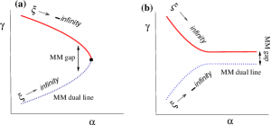
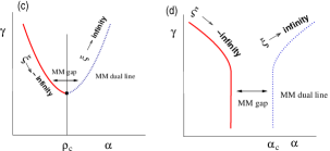
Figure 1: Possible phase boundaries (red thick line) and dual lines(blue dotted). (a,b) for the $\alpha$-phase with the shock forming at $x=1$ while (c,d) for the $\gamma$-phase with shock forming at $x=0$. In (a) and (c) the intersection of the shock phase boundary and the MM dual line produces a critical point marked by a filled square. No critical point in (b,d). The $\alpha$,$\gamma$ asymmetry depends on the relative values of $\rho_{L}$ and $\rho_{c}$.

The other length scale $w$ can be obtained from various limits of Eq. (4), the lengths differing by constant factors. From the asymptotic approach to the limits $\rho_{X}$, (X=o or s), $w^{-1}=(\rho_{s}-\rho_{\rm o})\Phi(\rho_{X})$, while for $\rho\approx\rho_{c}$, one gets $w^{-1}\sim\mid\rho_{\rm o}-\rho_{s}\mid/{\hat{S}}_{1}(\rho_{m})$. What is important to note is that for a given $\alpha$, the width is determined by the corresponding separation of the shockening and the dual line, to be called the MM-gap. The height $h$ of the shock on the shockening line is also equal to this MM-gap.

4.4 Condition for Critical point

In case the shockening transition line and the dual line intersect, then the intersection is at $\gamma=\rho_{c}$ with $w\to\infty$ as

$$w\sim\mid\rho_{\rm o}-\rho_{s}\mid^{-(2p-1)}\sim h^{-(2p-1)}.$$ (9)

Such a divergence is the signature of a critical point. The bulk phase transition from the $\alpha$-phase to the shock phase is first order because at the transition point $h>0$. On the other hand, the shock evolves from a zero height at the critical point so that it is a continuous transition. In case the two lines do not cross, there will be no critical point and the lines will span the whole phase diagram, symmetrically placed around $\gamma=\rho_{m}$ if $\Phi(\rho)=1$.

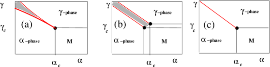
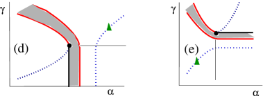
Figure 2: $\alpha-\gamma$ phase diagrams. (a,b,c) for $\rho_{L}=\rho_{m}$, (c) for $\rho_{L}>\rho_{M}$ and (d) for $\rho_{L}<\rho_{M}$. The critical points are represented by filled circles. The shaded region is the shock region. In (a) $q>p$. (b) $q=p$ while (c) has no non-conserving part. The MM dual lines are shown in (c) and (d) only. The filled triangles on the dual lines represent the point $(\rho_{L},\rho_{L})$ which is always on the dual line.

4.5 Phase diagrams

So far we have concentrated on the $\alpha$-phase only. A similar analysis can be done for the $\gamma$-phase for which the shock is formed at $x=0$. Here again there are two possibilities; the shockening and the dual lines either intersect at $\alpha=\rho_{m}$ or do not intersect but remain on two sides of $\alpha=\rho_{m}$. All the four possibilities are shown in Fig. 1. In these diagrams the lines at $\alpha=\alpha_{c}$ or $\gamma=\gamma_{c}$ or both remain special like the dual lines, representing boundary layer transitions.

Combining the two, we can now draw the global phase diagram. Combination of (a) and (c) of Fig. 1 one gets the type known for the $\rho_{L}=\rho_{m}$ ($K=1$) case of Ref. [2, 3, 8]. Similarly, (a) with (d) is known for $\rho_{L}>\rho_{m}$, while (b) with (c) will be the case for $\rho_{L}<\rho_{m}$. For $\gamma<\gamma_{c}=\rho_{m}$, on the $\alpha$-phase side, the U-type boundary layer renders an effective boundary value $\rho_{m}$ at $x=1$ and therefore the critical behavior continues for all $\gamma$. The shock on changing $\alpha$ evolves in height and shifts to $x=0$. On the $\gamma$-phase side, the response function $\chi_{\gamma}$ undergoes a change on crossing the line $\gamma=\rho_{m}$, even though the bulk density distribution changes smoothly. The line $\gamma=\rho_{m}$, like the MM dual lines, indicates a boundary transition, but in special situations it may develop into a bulk phase boundary also. The latter happens as $\rho_{L}\to\rho_{m}$.

The shape of the shockening curve near the critical point for $q=1$ is given by $(\gamma-\gamma_{c})\sim\mid\alpha-\alpha_{c}\mid^{1/2p}$. For $\gamma=\gamma_{c}=\rho_{m}$, the shock height vanishes on the shock side as $h\sim\mid\alpha-\alpha_{c}\mid^{\zeta^{\prime}}$ with $\zeta^{\prime}=1/(2p+1)$. Though the $p=1$ case is known in the literature, we have identified the whole class of multicritical points. All the exponents[3] associated with the shockening transition and the critical point can be determined in terms of $q,p$. These details will be reported elsewhere.

For $\rho_{L}=\rho_{m}$, our analysis via the duality yields the nature of the critical points. For $q=p$, the phase boundaries are similar to the $q=p=1$ case. However for $q>p$, the critical point is at $\alpha=\rho_{m},\gamma=\rho_{m}$. We show a new type of phase diagram for a particular case with $\rho_{m}=0.5$ in Fig. 2.

As one traverses the shock phase from one phase boundary to the other, the shock position goes from $x=1$ to $x=0$. Now, if the non-conserving part of the dynamics is removed, the shock region collapses on to a line as in Fig. 2(c). But the collapse also means that the shock is uniformly distributed over the entire length and the density is to be averaged over this distribution of shocks[10]. This yields the linear density profile one knows from exact solutions[4]. This also shows that the mean field theory puts a bias towards shock formations, so that a judicious use is called for in situations where shocks are not expected.

5 Summary

In summary, the MM duality theorem can be stated as follows: (a) Every shockening transition has a dual boundary transition. (b) If the two lines (the shockening transition and the dual line) intersect, there is a critical point. (c) The nature of the critical point is determined by the zeros of the $S_{i}$-functions. This theorem has been used to predict the behavior of a class of multicritical points in the steady state phase diagram of nonequilibrium transport. Our conclusion is that all microscopic perturbations need not be relevant to the phase diagrams. The microscopic dynamics needs to be analyzed for the nature of the zeros of the $S_{i}$ functions and the values of $q,p$. Those interactions or rules that change the density parameters $\rho_{L,m}$ without change in $q,p$, can be grouped into the same class. Perturbtions within the class will only make cosmetic changes in the phase diagram. We have shown a few examples of possible multicritical phase diagrams. New classes can be generated by including extra features of $S_{i}$’s.

References

- [*] email:somen@iopb.res.in
- [1] T. Liggett, Interacting Particle Systems: Contact, Voter and Exclusion Processes (Springer-Verlag, Berlin, 1999)
- [2] S. Mukherji and S. M. Bhattacharjee, J. Phys. A 38, L285 (2005).
- [3] S. Mukherji and V. Mishra, cond-mat/0510129.
- [4] B. Derrida et. al., J. Phys. A 26, 1493 (1993); G. Schütz and E. Domany, J. Stat. Phys. 72, 277 (1993).
- [5] G. Tripathy and M. Barma, Phys. Rev. Lett. 78, 3039 (1997); Phys. Rev. E 58, 1911 (1998).
- [6] M. R. Evans et. al., Phys. Rev. Lett. 74, 208 (1995); J. Stat. Phys. 80, 69 (1995).
- [7] J. Krug, Phys. Rev. Lett. 67, 1882 (1991); J. S. Hager et. al., Phys. Rev. E 63 056110 (2001).
- [8] A. Parmeggiani, T. Franosch and E. Frey, Phys. Rev. Lett. 90, 086601 (2003); cond-mat/0408034; M. R. Evans, R. Juhasz and L. Santen, Phys. Rev. E 68, 026117 (2003).
- [9] B. K. Chakrabarti, cond-mat/0603839.
- [10] I thank P. K. Mohanty for discussions on this point.